Synopsis

Keywords: Physics & Engineering: Physics, Contrast mechanisms: Relaxometry

The utility of MRI depends on the information carried by the contrast between different tissue types. This contrast can stem from MR-independent properties, like proton density, water diffusion or magnetic susceptibility, but is typically based on MR relaxation parameters, T₁, T₂ or T₂^*. All of these depend on the field strength. To compare data acquired at different fields, some understanding of these dependencies is necessary. In this presentation, the basic physics of relaxation mechanisms and their field dependence will be discussed. In addition, example data on relaxation measurements in brain imaging at various field strengths will be presented.

Introduction

Useful information in MR images stems for some form of contrast that allows differentiation between tissue types or for example between diseased and normal tissue. Contrast in the images, that is differences in signal intensity from one area to the next, can have a number of sources. Some are properties of the scanner, extrinsic to the object, and as they don't have bearing on the object, should be removed as much as possible from the created images. These external factors include the B0 (main magnetic field) and B1 (RF field) inhomogeneities. In general, magnets are sufficiently homogeneous that the former can be ignored, while the latter is typically removed from the images by for example dividing by a (RF) coil sensitivity profile acquired in a reference scan. Intrinsic sources of contrast can be basic properties of the object like the proton density, diffusion, magnetic susceptibility or chemical composition. MR images can be made sensitive to one of these, but as these are basic properties (similar to weight or the length), they are inherently not field dependent. Their effects however can be, as for example the susceptibility-induced phase scales with B0. Finally, there are intrinsic MR properties, in particular the relaxation parameters: T1, T2, T2*, representing the longitudinal, the irrecoverable transverse and total transverse relaxation times. T1 is the exponential decay time constant for the longitudinal magnetization (Mz) to relax to its equilibrium value, T2 and T2* refer to the decay constant of transverse (Mx & My) magnetization. The relaxation processes are often characterized by their rates, which are the inverse of the time constants. The distinction between external and internal sources shifts a little when considering only part of an object, for example one region of interest or one organ in the body. When imaging the brain, the rest of the body is external in this context. The body parts external to the brain will modify the magnetic field, so that the B0 inhomogeneity at the location of the brain is no longer negligible.

Theory

Relaxation rates can be calculated for some simple cases, as in for example a homogeneous medium. In this case, the only source of relaxation is the interaction between identical molecules. For this interaction to result in a change of the proton magnetization, the local field at the position of one proton spin from a neighboring spin has to fluctuate (at the precession (Lamor) frequency). These fluctuations can come from a change in the magnetic state (a spin flip in quantum mechanical terms) or from motion. T1 relaxation requires a change in the sum of the (magnetic) energy of all the spins, which means only the motion induced mechanism can play a role, coupling the magnetic and kinetic energy of the system (hence the term ‘spin-lattice’ relaxation). For T2 relaxation, direct spin-spin interaction can play a role, the fluctuating field of the neighboring spins can result in phase dispersion. Quantum mechanical treatment of the above results in [1,2]:

$$ R_1=\frac{1}{T_1}=\frac{3}{10}\frac{\gamma^4\hbar^2}{b^6}(\frac{\tau_c}{1+\omega^2\tau_c^2}+ \frac{4\tau_c}{1+4\omega^2\tau_c^2})$$ $$R_2=\frac{1}{T_2}=\frac{3}{20}\frac{\gamma^4\hbar^2}{b^6}(3\tau_c+ \frac{5\tau_c}{1+\omega^2\tau_c^2}+ \frac{2\tau_c}{1+4\omega^2\tau_c^2})$$

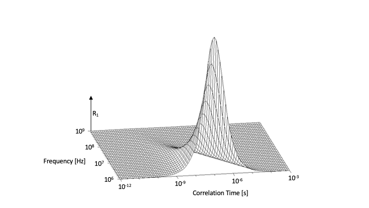
Where b is the inter-proton distance, $$$\omega$$$ the NMR frequency, and $$$\tau_c$$$ the correlation time. The equation for R1 is illustrated in Fig 1. The correlation time is the time scale of the motion of the interacting spins. For a correlation time short compared to the inverse of the frequency, the interactions are ineffective as the spins don’t have enough time to rotate a significant amount (the angle of rotation being $$$\tau_c \omega$$$). For much longer times, the fluctuations do not have sufficient power at the required frequency. So only for $$$\tau_c \omega \approx 1$$$ is there an effective T1 relaxation possible. While the T2 follows the same overall pattern, for long correlation times the frequency independent ('secular') term can result in a strong relaxation. For water, the correlation time is in the order of 1 ps, fast compared to NMR frequencies ($$$ \tau_c << 1/\omega$$$), resulting in long relaxation times with little field dependence, and T2 equal to T1. For solutions of larger molecules (proteins) in water, the correlation time of the water mobility relative to protein molecules can be in the order ms, resulting in strong relaxation effects at low field and a strong field dependence with a transition to slow T1 at higher field, but a significant, field independent T2 effect. For the slow protein motion to have an effect on the surrounding water, the two have to interact. This can be by water temporarily getting trapped/bound to the protein surface and exchanging with the ‘free’ water, or by some form of exchange between (proton) spins on the protein and surrounding water. Exchange is also important for the influence of lipids, which make up cell membranes, some intra cellular structures and, most prominently, the myelin sheath in white matter. The abundant protons on backbone of the semi-solid lipids strongly couple with each other with little motion, resulting in a short T2 (10-20 ms) and spin diffusion, which is the transport of magnetization along the lipid chain. Effective T1 relaxation happens mostly in the CH3 end groups, which have rotational mobility. The magnetization exchanges with water magnetization at the polar headgroups. The relaxation in the lipids acting through this exchange is the dominant source of T1 relaxation in white matter and source of contrast with the gray matter.

The classical definition of T2, as used in the Bloch equations, refers to a homogeneous medium, such as a pure liquid or a homogeneous solution of small molecules. Being homogeneous in the strict sense means the parameters do not vary in space, and all spins follow the same evolution. If we consider B0 inhomogeneity, due to variations in susceptibility, and image such a system, the spins getting added into the signal of one voxel can now have different frequencies, resulting in phase dispersion. This results in a form of signal decay in addition to the T2 of the substance being imaged. The combined effect is characterized by T2*, the decay time constant observed in a gradient echo image. As the inhomogeneity increases with B0, so does the R2*. The shape of the decay is not necessarily exponential and depends on the distribution of inhomogeneity within the voxel. The phase dispersion can be reversed by applying a refocusing pulse, resulting in a spin echo at the time point when all the spins come back into phase. The amplitude of the signal at the spin echo is governed by the T2, the decay of the transverse magnetization that is not reversible as it is due to random (on the time scale in a typical spin echo) molecular interactions. A complication arises when we consider diffusion in addition to the B0 inhomogeneity. Diffusion means the spins randomly move between the first and second half of the spin echo formation, and so the phase accumulation due to the inhomogeneity in these two halves do not necessarily cancel anymore, resulting in additional signal loss. The amount of signal loss relates to the amplitude of the inhomogeneity on the scale of the average distance the spins will diffuse. As the diffusion distance increases over time, the decrease in spin echo amplitude (in addition to the T2 decay) is dependent on the echo time of the spin echo. Or in a multi-spin echo sequence, on the spacing of the refocusing pulses. As it is difficult to separate this diffusion related decay from T2 as used in the Bloch equations or the equation above, it is frequently included into an effective T2. The diffusion attenuation is given by: $$$\gamma^2g^2TE^3D/12$$$, where $$$g$$$ is the local gradient, TE the echo time and D the diffusion coefficient. As the gradient scales with B0, this effect scales with B02. However, for inhomogeneities on a spatial scale smaller than the diffusion length, the averaging effect of the diffusional motion can reduce this to a linear dependence.

Examples

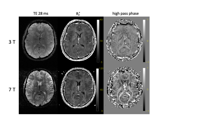
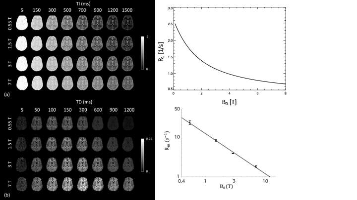
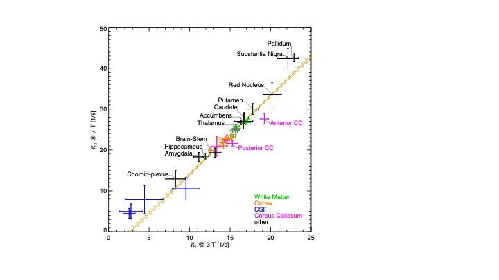
Several examples of field dependence are shown in the Figures 2-4. Figure 2 shows the comparison of gradient echo data acquired at 3 T and 7 T (on the same subject, approximately the same slice). The increase in contrast in the magnitude (at the same echo time), and in the phase is readily apparent. The phase data was high pass filtered to remove the slow varying background. The R2* fitted to the series of data at different echo times quantifies the field dependence.
Figure 3 shows the results of inversion and saturation recovery experiments, comparing fields from 0.55 to 7 T (data and part of the figure for [3]). The combined data allows for estimation of R1s, exchange and pool size parameters of a two pool model, which is essential to describe the T1 relaxation of tissue water that is in exchange with the semi-solids (mostly lipids) in the tissue. Figure 4 shows the results of R2 measurements at 3 T and 7 T, presented as the averages in various brain ROIs. The linear relation of R2 values between the two field strengths suggests an overall linear dependence, which is confirmed when considering R2 values reported in other studies as well.

Further Study

There are many papers on the subject of field dependent relaxation. Giving an overview of this extensive literature would be far outside the scope of this abstract, but please refer to the papers in the reference list for some suggested starting points.

Acknowledgements

No acknowledgement found.