MRI System Engineering
1MRIEngT, LFMI,NINDS, NIH, Bethesda, MD, United States
Synopsis
Keywords: Physics & Engineering: Hardware, Physics & Engineering: High-Field MRI, Physics & Engineering: Low-Field MRI
The aim of this presentation is to review the main hardware components in the MRI system and its engineering based on MRI physics.Introduction
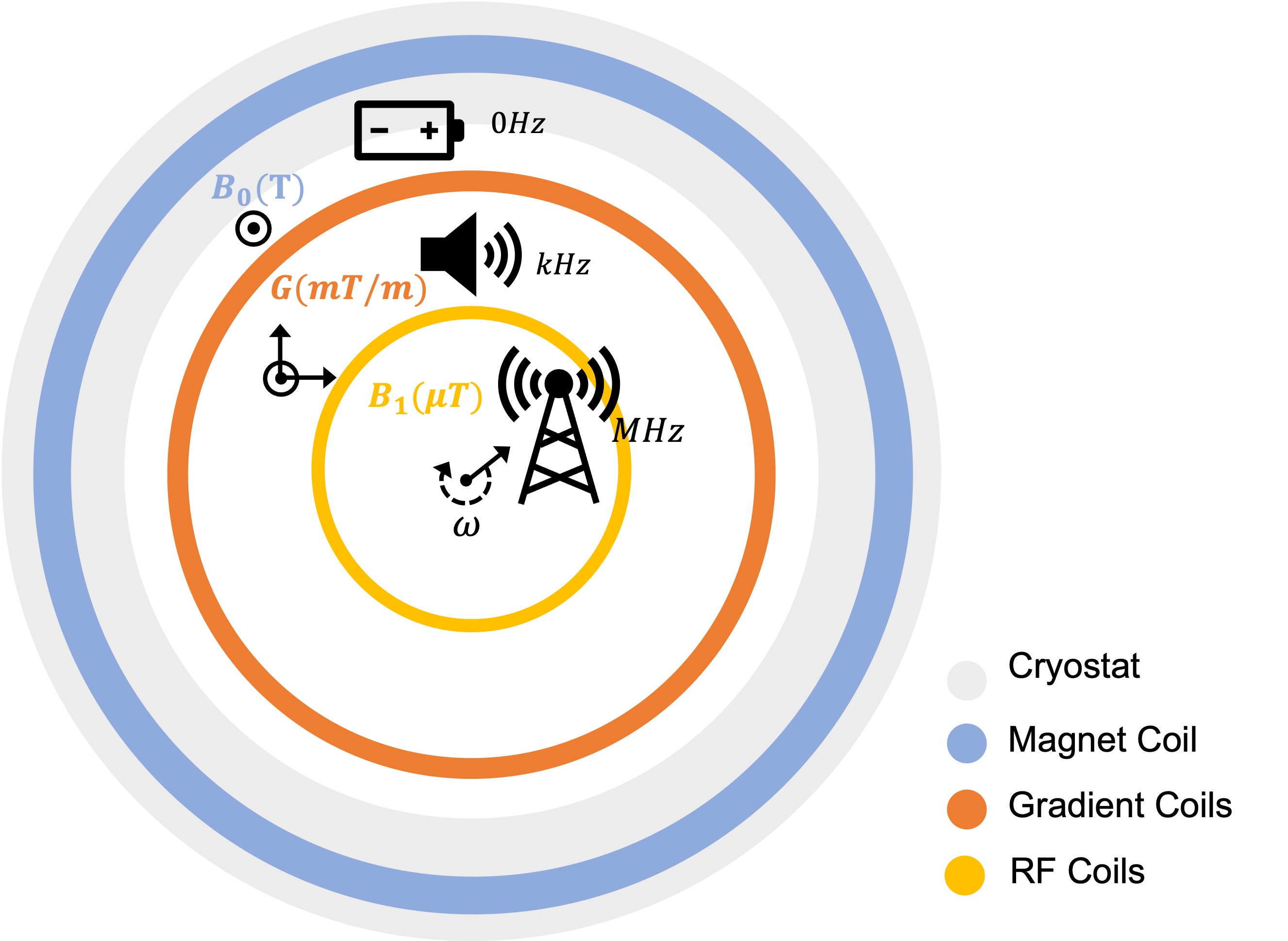
In MRI a very large magnet generates a strong static magnetic field (B0) (>10,000 x Bearth) to align the nuclear magnetic moments in the body which are otherwise in random orientation. This creates a bulk nuclear magnetisation (M0) proportional to the static field and nuclear spin density. To detect a particular nucleus, a high-power RF pulse excitation with angular frequency equal γB0 (Larmor frequency, γ : gyromagnetic ratio) is applied by a transmit (Tx) coil with axis (in x-y plane) perpendicular to B0 (z-axis). This generates a small magnetic field B1 that rotates at the same speed as the spins around B0 perturbing M0 from its equilibrium state (precessing around B0) to precess, only temporarily, around B1 field (in the transverse plane). After this pulsed excitation, M0 returns back to its equilibrium state aligned with B0. This free precession back to equilibrium induces a time variant voltage (ε) (MR signal) on a tuned receive (Rx) coil with axis also perpendicular to B0 (could be same Tx coil). The amplitude and transient response (oscillating at the Larmor frequency) of the magnetization depends on tissue relaxation constants (T1, T2, T2*) and nuclei spin density (ρ). The magnetization precession frequency is proportional to the static field; therefore, the MR signal can be spatially encoded in the frequency domain by well-defined varying magnetic field gradients ($$$\vec{G}$$$). Conventionally, field gradients in three directions (x, y, z) can be generated by three sets of coil arrangements that are concentrically located inside the magnet coil. A linear relationship between precession frequency and a spatial coordinate makes possible the generation of an image by a simple Fourier transform. All events involved in the generation of this image (RF excitation, gradient encoding and signal acquisition) are controlled by the MRI pulse sequence executed in the scanner console which communicates with all system hardware. An axial representation of the MRI system and fields is shown in Figure 1.Superconducting Magnets
Most MRI magnets today are built with several kilometers of superconducting wire, mostly niobium-titanium (Nb-Ti) and niobium-tin (Nb3-Sn). These low temperature superconductors (LTS) need to be kept at temperatures as low as 2 K. This requires a cryogenic system with large amount of liquid helium (He), and liquid nitrogen (N)1. Because in MRI we want image contrast to be associated to tissue properties, we need extremely high magnetic field homogeneity ( ΔB0 < 1 ppm) over a spherical volume (e.g. DSV= 30 cm ). This stringent homogeneity specification differentiates these magnets from those with similar strength used in particle accelerators and nuclear fusion. In search of higher spatial resolution, higher signal to noise ratio (SNR) and higher signal contrast (CNR), stronger magnets are being developed for both human and animal studies. Today there are human MRI systems up to 11.7 T in operation and up to 20 T in developing stage. Pushing MRI to higher field strengths requires new superconducting materials2. There is active research in building magnets with high temperature superconductors (HTS)3 which present superconductivity at higher temperatures and higher current densities at standard cryogenic temperatures. Advanced engineering of the MRI cryogenic system, led to the development of zero boil-off magnets as well as almost helium-free (few liters) MRI systems4 . This is important to overcome the decreasing supply and increasing price of He. Note that HTS can be kept at temperatures close to or above that of liquid nitrogen (> 77 K), eliminating the need for liquid He in the cryogenic system. In addition to the magnet coil, an MRI system can have active B0 shielding coils, also built from superconducting wire, located at both ends of the magnet coil to reduce stray fields outside the bore. To correct for unavoidable bulk B0 inhomogeneities, passive shimming can be performed on site by the arrangement of small ferromagnetic parts5. To compensate for B0 inhomogeneities introduced in the MRI experiment, dynamic electrical shimming can be performed through additional wired loops driven independently to generate different field harmonics6. Electrical B0 shimming hardware can be assembled with gradient coils and/or customized RF hardware7,8.Gradient Coils
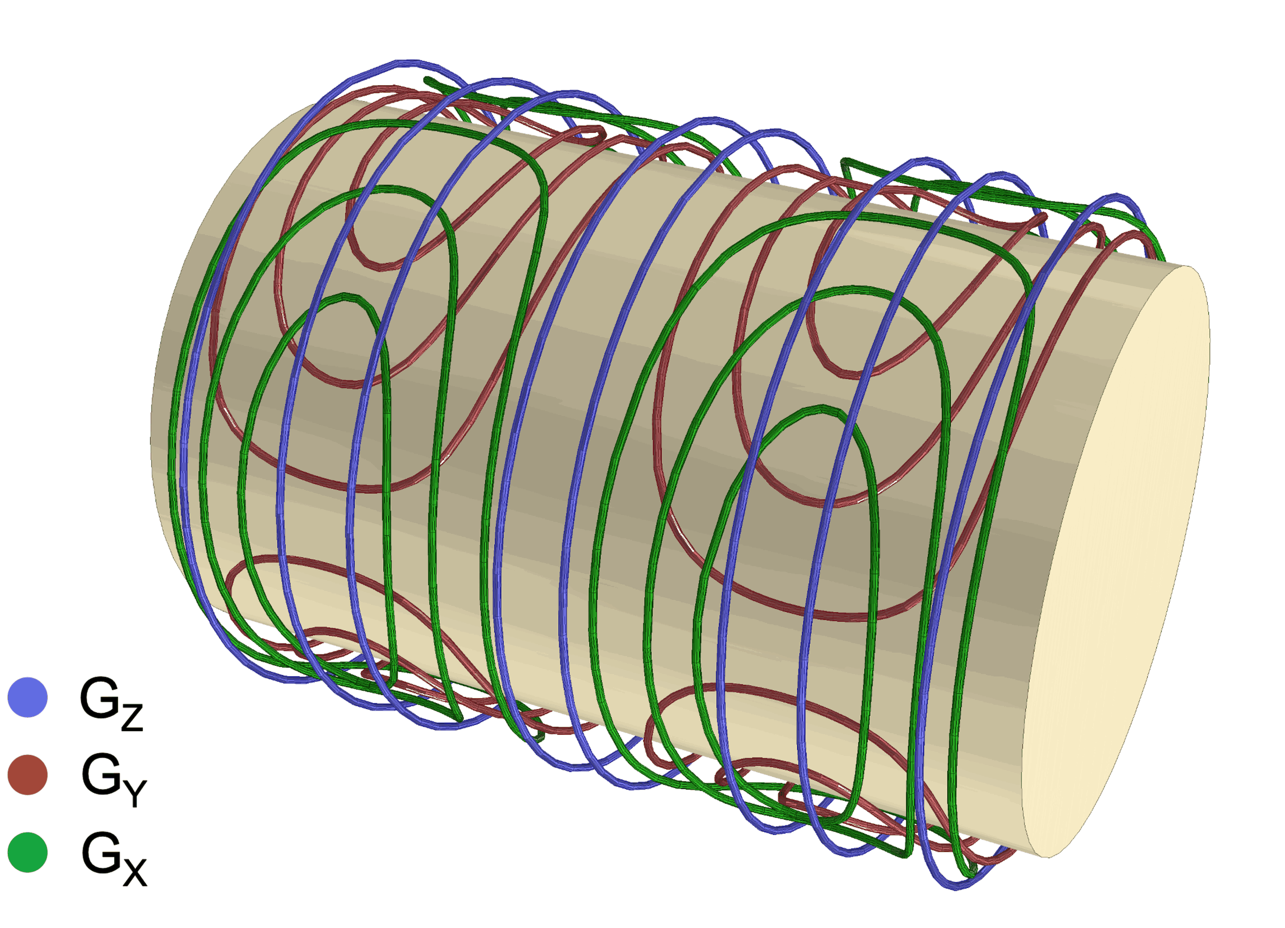
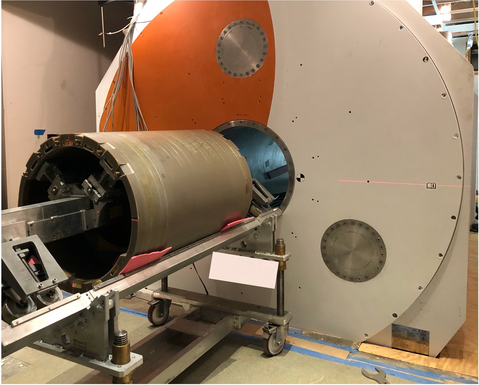
MRI scanners have 3 sets of gradient coil arrangements integrated into an annular layer inside the bore of the main magnet winding. Each of these coils generate an independent spatial field change along x, y and z (Gx, Gy, Gz). The field change is linear in the imaging volume. The z-gradient is generated by sets of circular loop pairs coaxially arranged along the z-axis and symmetrically spaced from the z=0 plane. The currents on each side of the pairs run in opposite directions such as to increase (parallel field) or decrease (anti-parallel field) the total magnetic field. In most MRI scanners today, the x-and y-gradients are generated by finger-print coils based on the Golay configuration9 and laid on a cylindrical surface concentrically to the magnet coil. Both gradient coil layouts are similar but with axis rotated 90 degrees (Figure 2). As in the z-gradient coil, loops are spatially symmetric and driven by anti-symmetric currents such as to generate fields in parallel and antiparallel with B0 across x and y direction. These coils have an additional coil layer that minimizes eddy currents in surrounding conductive surfaces especially the cryostat. Each of these gradient coils is independently driven by a power amplifier. In order to generate enough field change and spatially encode the nuclear spin resonance, gradient coils can be driven by currents as high as 900 A10. Gradient encoding only happens in a portion of the imaging cycle, which can be as short as few milliseconds, where gradient coils are switched on-off at frequencies in the kHz well inside the audio range. Because these large coils have inductances on the order of thousands of microhenries, the fast switching of the currents induces voltages on the order of thousands of volts. Gradient hardware in the MRI scanner can handle power levels on the order of MW, higher than any other hardware (like RF and shimming hardware) during an MRI scan. At kHz frequency range, amplifier losses can be minimized by using ultra-high-power efficient switch-mode amplifiers using Pulse-Width-Modulation (PWM). Different from magnet coils, gradient coils are not built with superconductive wires, so at the high gradient currents, power dissipation in the wire can be on the order of several kW. This requires water cooling which is usually implemented by chilled water pipes in close contact with gradient coil wires. There is continuous optimization of the gradient hardware to achieve the highest SNR and resolution possible11. At ultra-high field (≥7 T), an additional challenge is the minimization of magnet-gradient interaction to ensure system stability12,13. Figure 3 shows the installation of a gradient assembly in an ultra-high field MRI magnet.RF Hardware
Of all the MRI hardware, RF coils are the most accessible and customizable hardware to improve image quality for a specific application. In MRI scanners with field strengths up to 3 T, RF transmission is integrated in the scanner bore through the body coil. This volume coil has a cylindrical shape and it is built from multiple rungs distributed along the cylindrical surface and aligned in the direction of the static field (z-axis). Both end-ring segments connecting each rung are capacitively or inductively coupled to the next rung. This “birdcage” structure has 2 ports that are located 90 degrees azimuthally from each other and receive high voltages with same amplitude but with a 90 degree phase delay14. These voltages generate a sinusoidal current distribution along the rungs that creates a time variant magnetic field (B1), on resonance and rotating with the nuclear magnetization. Therefore this Tx hardware can generate a very homogenous excitation of the magnetization in a well-defined volume. The body coil can be used as a Tx only or as a Tx-Rx coil. It has been shown that receiving the MR signal with an array of surface loops, instead of a volume coil, provides higher SNR and image acceleration by skipping acquisition lines and taking advantage of coil spatial information. This approach is known as parallel imaging15,16. Most imaging protocols today use a volume coil as a Tx only coil and a Rx array with as many as 128 elements17. At higher field strengths the shorter excitation wavelength compromises the homogeneity achieved with this coil architecture, and other Tx approaches should be considered. To achieve higher homogeneity of the excitation field, an array of Tx coils can be independently controlled18-20. This method is known as parallel transmission (pTx). Some ultra-high field scanners have pTx interfaces, up to 16 channels, implemented in their control. The technology for these ultra-high field systems continues to evolve to compensate for field inhomogeneities caused by tissue properties of the body and to automate methods for obtaining high quality images while ensuring patient safety. At low field the excitation field can be perfectly homogenous, but the engineering challenge is to optimize Rx hardware to compensate for the loss in signal and reduced sample loading21.System Control
The user interface, sequence and coil files are located in a host computer which communicates to all hardware through a controlled area network. Here the user can edit protocols, load sequences, manage the exam database, monitor system error/warnings and SAR. In most MRI systems, the host sends instructions to the hardware control (gradient, RF, shimming) for the execution of MRI sequences, and communicates with the measurement and reconstruction system, which receives a digitized version of the Rx signals to compute the image. Synchronization of all signals and processes is commanded by the hardware control. This hardware is located in cabinets in the electronics room. Gradient, shimming, and RF amplifiers are also normally located in this room and connected to all coils in the MRI suite through a penetration panel in the scanner shield (Faraday cage). The MRI control receives information from monitoring hardware and sensors (e.g. RF directional couplers, gradient temperature and current sensors, cold head sensors, etc.) to ensure system performance and patient safety. In addition to the monitoring of the status of the multiple hardware components in the MRI systems, the MRI control can trigger and receive information from physiological monitoring hardware. The level of integration of this hardware into the MRI system varies across scanner vendors.Acknowledgements
References
1- Cosmus TC, Parizh M. Advances in Whole-Body MRI Magnets. IEEE Trans. Appl. Supercond. 2011;21(3):2104-2109.
2- Parizh M, Lvovsky Y, Sumption M. Conductors for commercial MRI magnets beyond NbTi: requirements and challenges. Supercond Sci Technol. 2016;30(1):014007.
3- Bai H, Bird MD, Cooley LD, et al. The 40 T Superconducting Magnet Project at the National High Magnetic Field Laboratory. IEEE Trans. Appl. Supercond. 2020;30(4):1-5.
4- Ackermann RA, Menteur P, Dhar M. Very efficient heat exchanger for cryogen free mri magnet. August 2014. US Patent 20140243205A1
5- Hoult DI, Lee D. Shimming a superconducting nuclear-magnetic-resonance imaging magnet with steel. Rev. Sci. Instrum. 1985;56:131-135.
6- Golay MJE. Field Homogenizing Coils for Nuclear Spin Resonance Instrumentation. Review of Scientific Instruments. 1958;29(4):313-315.
7- Juchem C, Nixon TW, McIntyre S, Boer VO, Rothman DL, de Graaf RA. Dynamic multi-coil shimming of the human brain at 7T. J Magn Reson. 2011;212(2):280-288.
8- Stockmann JP, Witzel T, Keil B, et al. A 32-channel combined RF and B0 shim array for 3T brain imaging. Magn Reson Med. 2016;75(1):441-451.
9- Golay MJE. Magnetic field control apparatus. June 1957:US Patent 3,515,979.
10- Smith F. The gradient system. Proc Intl Soc Mag Reson Med 2013;21.
11- Gudino N, Littin S. Advancements in Gradient System Performance for Clinical and Research MRI. J Magn Reson Imaging. 2023;57(1):57-70.
12- Winkler SA, Schmitt F, Landes H, et al. Gradient and shim technologies for ultra high field MRI. NeuroImage. 2018;168:59-70.
13- Roemer PB, Rutt BK. Minimum electric-field gradient coil design: Theoretical limits and practical guidelines. Magn Reson Med. 2021;86(1):569-580.
14- Hayes CE, Edelstein WA, Schenck JF, Mueller OM, Eash M. An efficient, highly homogeneous radiofrequency coil for whole-body NMR imaging at 1.5 T. J Magn Reson (1969). 1985;63(3):622-628.
15- Pruessmann KP, Weiger M, Scheidegger MB, Boesiger P. SENSE: sensitivity encoding for fast MRI. Magn Reson Med. 1999;42(5):952-962.
16- Griswold MA, Jakob PM, Heidemann RM, et al. Generalized autocalibrating partially parallel acquisitions (GRAPPA). Magn Reson Med. 2002;47(6):1202-1210.
17- Gruber B, Stockmann JP, Mareyam A, et al. A 128-channel receive array for cortical brain imaging at 7 T. Magn Reson Med. August 2023.
18- Katscher U, Börnert P, Leussler C, van den Brink JS. Transmit SENSE. Magn Reson Med. 2003;49(1):144-150.
19- Zhu Y. Parallel excitation with an array of transmit coils. Magn Reson Med. 2004;51(4):775-784.
20- Katscher U, Börnert P. Parallel RF transmission in MRI. NMR in Biomed. 2006;19(3):393-400.
21- Webb A, O’Reilly T. Tackling SNR at low-field: a review of hardware approaches for point-of-care systems. Magn Reson Mater Phy. 2023;36(3):375-393.
Figures