Signal & Noise Considerations Across B0s
1A.A. Martinos Center MGH, Charlestown, MA, United States
Synopsis
Keywords: Physics & Engineering: Physics
The signal-to-noise ratio is one of the most important determinants of our ability to extract information from a measurement in that it expresses the signal measurement’s relative uncertainty. Improving it is a frequent target of technical development and SNR is constantly monitored as a quality assessment. This seemingly simple ratio of the signal level to its uncertainty or “noise” level, would appear a simple and well-defined metric but is more difficult to measure than one would think and it is critical to understand how each component (signal and noise) is modulated by experimental parameters.Introduction
“A measurement without knowledge of its uncertainty is completely meaningless” – Walter LewinThe signal-to-noise ratio is one of the most important determinants of our ability to extract information from a measurement in that it expresses the signal measurement’s relative uncertainty. Improving it is a frequent target of technical development and SNR is constantly monitored as a quality assessment. This seemingly simple ratio of the signal level to its uncertainty or “noise” level, would appear a simple and well-defined metric but is more difficult to measure than one would think. It is critical to understand how each component (signal and noise) is modulated by experimental parameters such as field strength, coil geometry, and imaging parameters and to note that the noise, for example in receive coil channels, is not always independent, and that image reconstructions can render the noise non-identically distributed (not IID). This talk discusses the source of both signal and noise in the MR measurement, how they vary, and how to measure SNR in an array image where simplistic estimates of noise, such as measuring noise levels in signal-less areas outside the body do not accurately characterize the noise in the parts of the image you care about.
Detected signal; S
We are interested in the signal S induced by a small voxel at position (x,y,z). This is subtly different from the total signal from the object. For nearly all MRI scanners, S is the signal voltage from the processing nuclear magnetization detected via Faraday Induction. In a Faraday Inductive measurement, the precessing nuclear spin magnetization creates a time-varying magnetic field that threads the conductive loop of the Rx coil. The spatial integral of this field over the coil area is the flux, Φ(t). The precessing flux after a 90o excitation is, Φ(t) = Φ0 cos(ω0 t), where Φ0 is the equilibrium flux which is related to the equilibrium magnetization, M0, in the voxel volume via Φ0 = c M0, where c is a constant that captures the geometric integral, and ω0 is the Larmor frequency (e.g. 42.577 MHz for protons at 1T). Faraday’s law tells us that a time-varying flux will induce an electromotive force in that loop; EMF = -dΦ/dt, the same principle as a dynamo or electrical generator. This EMF voltage is stepped up via a lossless transformer (the coil matching network), amplified with the preamplifier, and recorded as the voltage signal S by the scanner’s receiver. Thus, the signal before preamplification is: S(t) = Φ0 ω0 sin(ω0 t). The receiver will demodulate the signal, leaving only S = Φ0 ω0 = c M0 ω0. We immediately see that the signal voltage grows with the square of B0 since both M0 and ω0 are proportional to B0, i.e. (M0 = cB0, and ω0 = γ B0), while c is a geometric constant. A 7T scanner has 22x the signal voltage of a 1.5T scanner (which has consequences for the receive chain).We can go one step further and express the geometric constant in terms of the efficiency the receive coil would have as a transmitter. Namely, the reciprocity theorem tells us that c is proportional to the transverse field, Bt, that the coil would produce if an ampere of current flowed in it. Note that many fields focus on the signal power, and form the SNR as a power ratio, but in MR the image intensity is proportional to the detected voltage and therefore we focus on a voltage SNR ratio.
Detected noise; σ
Electrical losses in a lossy material manifest themselves as voltage fluctuations (Johnson noise). The spectral density of this noise is white (constant in frequency) and the mean squared voltage in a resistor R is <V2> = 4kBT Δf R where kB is the Boltzmann constant T is the temperature, and Δf is the bandwidth of frequencies allowed into the measurement. So the noise, Vnoise = SQRT(4kBT ΔfR).It is no surprise that losses in the wire and other electrical components contribute to the resistance, R. But most people are surprised to learn that sample losses actually dominate R for frequencies above about 50 MHz. The body is a lossy conductor and the fluctuation-dissipation theorem (FDT) tells us that all losses, even those incurred through inductive coupling contribute Johnson noise. Another way to view it is that the ions in the body are thermally driven in random motion and some of that motion forms loops of current that happen to oscillate at the Larmor frequency. Their magnetic fields are therefore detected just like those of the spins.
Breaking the losses the coil experiences, R, into contributions from the copper losses in the loop, Rcopper, and losses due to induced currents in the lossy tissue, Rbody, we have R = Rcopper + Rbody. Measuring the coil quality factor (Q = ωL/R) with and without the body-load present informs us of the relative strength via the “Q ratio” Qunloaded / Qloaded = 1 + Rbody / Rcopper. Thus a quick Q ratio immediately tells us the relative contribution of body losses and copper losses and thus our dominant noise source. Kumar et al (2009) note that the voltage SNR is expected to degrade by the square root of this factor on loading the coil. This simple measure immediately tells the coil engineer what the benefit might be gained from improved conductors, and it is sadly meager for most high-field coils. For example, a typical Q ratio of 7 (for, say, a 3T 8cm loop), gives Rbody / Rcopper = 6, and eliminating the copper noise (by making the coil superconducting) would increase the SNR by a factor of 17%.
So, far from thinking that body noise dominance is a bad thing, we think about it as a positive indication that the coil designer succeeded in reducing component losses to an insignificant level. Alternatively, if the coil is good at picking up the ionic fluctuations in the body at the Larmor frequency (body load noise), then it will also be good at detecting spins. If you want to go beyond the Q ratio measurement, you calculate the body loss by integrating the square of the induced electric field over the body using EM simulation software and a numerical body model with assigned conductivities. A final loss mechanism is the radiated power from the coil, which is typically tiny for receiver coils. Radiative losses scale as the fourth power of the frequency and circumference.
The SNR equation
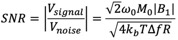
Putting together the above expressions for signal and noise leaves us the usual expression for MRI’s voltage SNR (see figure for equation) Where M0 is the total magnetization in the voxel (sometimes written as the product of a magnetization density and the voxel volume) and B1 refers to the transverse B1 generated per ampere of current in the Rx coil. The SQRT(2) comes from taking only one of the circular polarizations of the B1 field.Measuring SNR
Paradoxically, neither the Vsignal nor the Vnoise is easy to accurately measure in many cases! Drawing an ROI in the “signal region” and recording the average as “S” followed by a mean or SD measure in a “noise” region outside the object is the go-to method, but can lead to spectacularly incorrect results, especially for low SNR array coil images. And these days, almost all images are array coil images, and if the image is high-SNR, you probably don’t care about measuring it! An excellent outline of all the problems (and how to do it right) is found in Kellman 2005.One problem arises from the analysis of magnitude images, which causes the noise to always add as a positive offset to signal areas. Thus the average intensity in the “signal ROI” will be higher than it should be in areas with low SNR. In pure noise regions, the distribution of the noise is also changed from a Gaussian to a Rician distribution, and the SD value must be “corrected” to reflect the underlying Gaussian distribution of the complex data (Gudbjartsson 1995). The correction factor gets bigger for array coils (Kellman 2007, Triantafyllou 2011). Kellman 2007 concentrates on this and the other problems of measuring SNR in array coil images, such as the noise correlation between the channels, as well as taking into account the weights used in combining the array channels to form each pixel. The optimal combination should weight each pixel by its expected SNR before combination, but common methods like “root-sum-of-squares” combinations, take a short-cut that does pretty well in high SNR areas, but essentially weights noise by noise in low SNR regions (such as outside the object). The result is that the noise outside the object is poorly combined and a poor estimate of the noise inside the object (where we care…). In any case, the pixel weightings must be known to properly estimate the signal and noise in the combined image, and the individual channel data must be on hand (which is often not the case if you only have Dicom images.)
The final result of Kellman’s recipe is an SNR map in “SNR units” that should agree with an SNR map derived from the “Monte Carlo” or “time-series” method by which the image is taken multiple times and a signal average and SD is computed across the repeated measurements. The problem, of course, with the time-series method is that physiological processes such as motion may corrupt the SNR measure. Considerable effort has gone into exploring these thermal and physiological noise sources in time-series fMRI data and assessing how they scale with image SNR, field strength and coils (Kruger 2001, Triantafyllou 2005). Finally, it should be noted that accelerated imaging reconstructions, and modern reconstructions employing prior knowledge (such as compressed sensing and ML-based methods) all impact what happens to the noise. In conventional parallel imaging, one typically needs to compute the effect of the reconstruction on the noise maps of the individual channels. I.e. compute the g-factor map. Note the spatial pattern of noise enhancements by these reconstructions is far from uniform. Again, the individual channel’s complex data will be needed as well as an intimate knowledge of the reconstruction algorithm.
Ultimate SNR
Amazingly it is possible to compute the SNR expected from the best possible Faraday Induction detector array placed outside the body. (Ocali and Atalar 1998) To do this, one numerically computes the image data from a basis-set of detectors that spans the space of all possible electromagnetic field patterns. Thus, any array’s data can be expressed as a linear combination of this basis set. The optimal SNR map is formed from the linear combination that maximizes SNR. Typically this has been limited to simple object geometries like loading spheres and cylinders where the basis set has an analytical form, but it has also been extended to a realistic human head model at different field strengths.(Guerin 2017) Comparison of a measured SNR map to the ultimate SNR map is a good way to assess how much work the coil designer has ahead of him/her. The short answer is that arrays of 16 or more channels do well in the center of the head, but we have room for improvement at the periphery (Wiesinger 2005, Lattanzi 2010).Acknowledgements
No acknowledgement found.References
Constantinides CD, Atalar E, McVeigh ER. Signal-to-noise measurements in magnitude images from NMR phased arrays. Magn Reson Med. 1997 Nov;38(5):852-7. doi: 10.1002/mrm.1910380524. Erratum in: Magn Reson Med. 2004 Jul;52(1):219. PMID: 9358462; PMCID: PMC2570034.
Edelstein WA, Glover GH, Hardy CJ, Redington RW. The intrinsic signal-to-noise ratio in NMR imaging. Magn Reson Med. 1986 Aug;3(4):604-18. doi: 10.1002/mrm.1910030413. PMID: 3747821.
Gudbjartsson H, Patz S. The Rician distribution of noisy MRI data. Magn Reson Med. 1995 Dec;34(6):910-4. doi: 10.1002/mrm.1910340618. Erratum in: Magn Reson Med 1996 Aug;36(2):332. PMID: 8598820; PMCID: PMC2254141.
Guérin B, Villena JF, Polimeridis AG, Adalsteinsson E, Daniel L, White JK, Wald LL. The ultimate signal-to-noise ratio in realistic body models. Magn Reson Med. 2017 Nov;78(5):1969-1980. doi: 10.1002/mrm.26564. Epub 2016 Dec 4. PMID: 27917528; PMCID: PMC5532082.
Kumar A, Edelstein WA, Bottomley PA. Noise figure limits for circular loop MR coils. Magn Reson Med. 2009 May;61(5):1201-9. doi: 10.1002/mrm.21948. PMID: 19253376; PMCID: PMC2869245.
Kellman P, McVeigh ER. Image reconstruction in SNR units: a general method for SNR measurement. Magn Reson Med. 2005 Dec;54(6):1439-47. doi: 10.1002/mrm.20713. Erratum in: Magn Reson Med. 2007 Jul;58(1):211-2. PMID: 16261576; PMCID: PMC2570032.
Krüger G, Glover GH. Physiological noise in oxygenation-sensitive magnetic resonance imaging. Magn Reson Med. 2001 Oct;46(4):631-7. doi: 10.1002/mrm.1240. PMID: 11590638.
Le Ster C, Grant A, Van de Moortele PF, Monreal-Madrigal A, Adriany G, Vignaud A, Mauconduit F, Rabrait-Lerman C, Poser BA, Uğurbil K, Boulant N. Magnetic field strength dependent SNR gain at the center of a spherical phantom and up to 11.7T. Magn Reson Med. 2022 Nov;88(5):2131-2138. doi: 10.1002/mrm.29391. Epub 2022 Jul 18. PMID: 35849739; PMCID: PMC9420790.
Lattanzi R, Grant AK, Polimeni JR, Ohliger MA, Wiggins GC, Wald LL, Sodickson DK. Performance evaluation of a 32-element head array with respect to the ultimate intrinsic SNR. NMR Biomed 2010;23:142–151.
Ocali O, Atalar E. Ultimate intrinsic signal-to-noise ratio in MRI. Magn Reson Med. 1998 Mar;39(3):462-73. doi: 10.1002/mrm.1910390317. PMID: 9498603.
Triantafyllou C, Hoge RD, Krueger G, Wiggins CJ, Potthast A, Wiggins GC, Wald LL. Comparison of physiological noise at 1.5 T, 3 T and 7 T and optimization of fMRI acquisition parameters. Neuroimage. 2005 May 15;26(1):243-50. doi: 10.1016/j.neuroimage.2005.01.007. PMID: 15862224.
Triantafyllou C, Polimeni JR, Wald LL. Physiological noise and signal-to-noise ratio in fMRI with multi-channel array coils. Neuroimage. 2011 Mar 15;55(2):597-606. doi: 10.1016/j.neuroimage.2010.11.084. Epub 2010 Dec 16. PMID: 21167946; PMCID: PMC3039683.
Uğurbil K, Auerbach E, Moeller S, Grant A, Wu X, Van de Moortele PF, Olman C, DelaBarre L, Schillak S, Radder J, Lagore R, Adriany G. Brain imaging with improved acceleration and SNR at 7 Tesla obtained with 64-channel receive array. Magn Reson Med. 2019 Jul;82(1):495-509. doi: 10.1002/mrm.27695. Epub 2019 Feb 25. PMID: 30803023; PMCID: PMC6491243.
Wiesinger F, De Zanche N, Pruessmann K. Approaching ultimate SNR with finite coil arrays. In Proceedings
Figures