Introduction

When performing biomarker measurements, a common question is "what if I had performed my experiment differently?". In body diffusion-weighted MRI, selecting an appropriate diffusion encoding gradient scheme is crucial. Common options include trace-weighting (three orthogonal directions for rotationally invariant apparent diffusion coefficient [ADC]), single-direction (to reduce echo-times under isotropic diffusion assumptions), and multi-directional diffusion weighting (MDDW) with six or more directions for full tensor estimation, often overlooked in cancer applications [1]. Here, we propose Bayesian approaches to predict the difference in ADC measurements made using trace-weighting and single-direction schemes given data acquired using MDDW. This is validated through simulation studies and appears to demonstrate no systematic error in estimating this ADC bias.

Theory

Consider acquired data $$$y$$$ modelled by some likelihood function $$$p(y | \theta, X)$$$ given (unknown) model parameters $$$\theta$$$ and (known) experimental conditions $$$X$$$. We wish to determine the posterior distribution of estimated parameters $$$\widehat{\theta}'$$$ given different experimental conditions $$$X'$$$:
$$p(\widehat{\theta}'|y,X,X') =\int_{y'}\int_{\theta}p(\widehat{\theta}'|y',X')p(y'|\theta,X')p(\theta|y,X)\text{d}\theta\text{d}y'\quad\text{(1)}$$
Samples of $$$\widehat{\theta}'$$$ may be obtained using Markov Chain Monte Carlo (mcmc) techniques:
For $$$t\in\{1,\dots,N\}$$$:

1. $$$\theta_{t}\sim p(\theta|y,X)$$$
2. $$$y'_{t}\sim p(y'|\theta_{t},X')$$$
3. $$$\widehat{\theta}'_{t}=f(y'_{t},X')$$$

where $$$f(\cdot)$$$ represents the parameter estimator (e.g. maximum-likelihood); samples in step 1 may be generated by any Bayesian inference engine (Stan in our case [2]).

In this work $$$\theta = (\mathbf{D}, S_{0}, \sigma)$$$, where $$$\mathbf{D}$$$ denotes the diffusion tensor with trace($$$\mathbf{D}$$$) = $$$D$$$, $$$S_{0}$$$ the signal intensity without diffusion weighting, and $$$\sigma$$$ the standard-deviation of (assumed) homoscedastic noise. Experimental conditions are:

1. Trace-weighting, $$$X^{\dagger}$$$, resulting in ADC estimate $$$\widehat{D}^{\dagger}$$$.
2. Single-direction, $$$X^{*}$$$, resulting in ADC estimate $$$\widehat{D}^{*}$$$.
3. Six-directional MDDW, $$$X$$$, from which the posterior distribution $$$p(\mathbf{D}, S_{0}, \sigma|X, y)$$$ is to be sampled.

Throughout, we define bias as $$$\mathcal{B}=\frac{\widehat{D}^{\dagger}-\widehat{D}^{*}}{D}\times 100\%$$$.

Methodology

Simulations
Noisy MDDW data were sampled from a Rician distribution [3] for each combination of parameters: Fractional anisotropy $$$FA\in\{-1/\sqrt{2},-1/2,0,1/2,1/\sqrt{2},\sqrt{3}/2,1\}$$$, $$$SNR\in\{5,10,15,20,30,50\}$$$ and $$$D\in\{0.5,1.0,1.5,2.0\}$$$ $$$\times 10^{-3}$$$ mm²/s. The design matrix consisted of 3 b-values (50, 600 and 900) and a six-direction MDDW scheme with gradient directions $$$\{(0,-1,1),(0,-1,-1),(-1,0,1),(-1,0,-1),(1,-1,0),(-1,-1,0)\}$$$ (following normalization to unit length). $$$M=20$$$ diffusion tensors, $$$\mathbf{D}$$$, were generated for each combination of parameters by uniformly sampling eigenvectors on a unit sphere and assuming two eigenvalues are identical: $$$\lambda_{1}=\lambda_{2}=\lambda$$$ (negative $$$FA$$$ indicates where $$$\lambda>\lambda_{3}$$$), resulting in 3360 total simulations. In each simulation, $$$N$$$ = 4000 samples of estimated bias $$$\mathcal{B}_{est}$$$ were drawn using the MCMC algorithm detailed in "Theory". Furthermore, 4000 samples of the true bias $$$\mathcal{B}_{true}$$$ were generated by sampling directly from the likelihood function given the true parameters ($$$y'_{t}\sim p(y'|\mathbf{D}, S_{0}, \sigma,X')$$$):

Analysis
We approximate distributions of bias as kernel density estimates of respective samples:
$$
p(\mathcal{B})\approx\frac{1}{hN}\sum\limits_{t=1}^{N}\mathcal{K}\left(\frac{\mathcal{B}-\mathcal{B}_{t}}{h}\right)
$$
with $$$\mathcal{K}(u)=\frac{1}{\sqrt{2\pi}}e^{-\frac{1}{2}u^{2}}$$$ and $$$h$$$ estimated using Silverman's rule [4]. The overlap between distributions $$$\mathcal{B}_{true}$$$ and $$$\mathcal{B}_{est}$$$ for simulation $$$r$$$ is defined as [5]
$$
\Omega^{\delta}_{r}=\int\limits_{-\infty}^{\infty}\text{min}\left(p(\mathcal{B}_{true, r}),p(\mathcal{B}_{est, r})\right)\text{d}\mathcal{B}\quad\text{and}
$$
Furthermore, the overlap between pairs of distributions from simulations $$$r$$$ and $$$p$$$ within the same parameter combination is:
$$\Omega^{\Delta}_{r, p}=\int\limits_{-\infty}^{\infty}\text{min}\left(p(\mathcal{B}_{true, r}),p(\mathcal{B}_{true, p})\right)\text{d}\mathcal{B}
$$
Average overlaps for each parameter combination are then calculated as
$$
\left\langle\Omega^{\delta}\right\rangle=\frac{1}{M} \sum\limits_{r=1}^{M}\Omega^{\delta}_{r}\quad \text{and}\quad\left\langle\Omega^{\Delta}\right\rangle=\frac{1}{M(M-1)/2}\sum\limits_{r=1}^{M-1}\sum\limits_{p=r+1}^{M}\Omega^{\Delta}_{r, p}
$$
We define a within-group overlap similarity index as
$$
\text{OSI}=\frac{\left\langle\Omega^{\delta}\right\rangle}{\left\langle\Omega^{\delta}\right\rangle+\left\langle\Omega^{\Delta}\right\rangle}
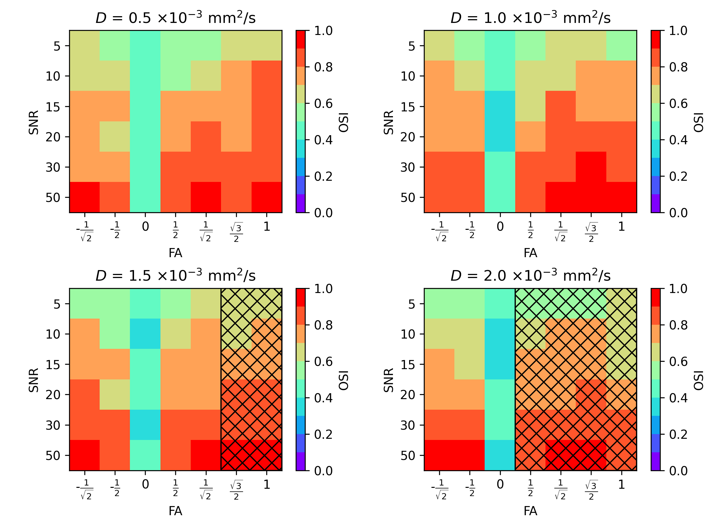
$$
where OSI=1 represents an ideal agreement, whilst OSI=0 represents very poor agreement between $$$\mathcal{B}_{true}$$$ and $$$\mathcal{B}_{est}$$$.

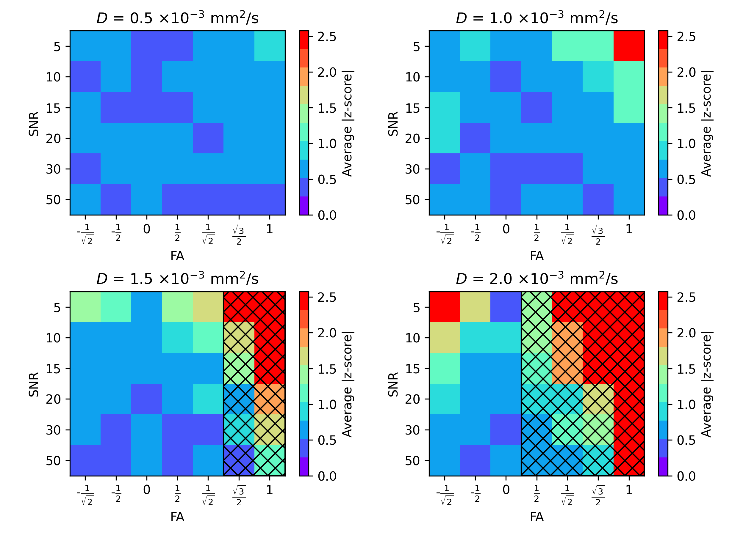
Lastly, the theoretical bias of mean diffusivity between trace-weighted and single-directional encoding schemes may be found as $$$\mathcal{B}_{theo}=\frac{2}{3}\left(D_{xy},D_{xz},D_{yz}\right)$$$; the average absolute z-score of this value from $$$\mathcal{B}_{est}$$$ data was also derived for each parameter combination.

Results

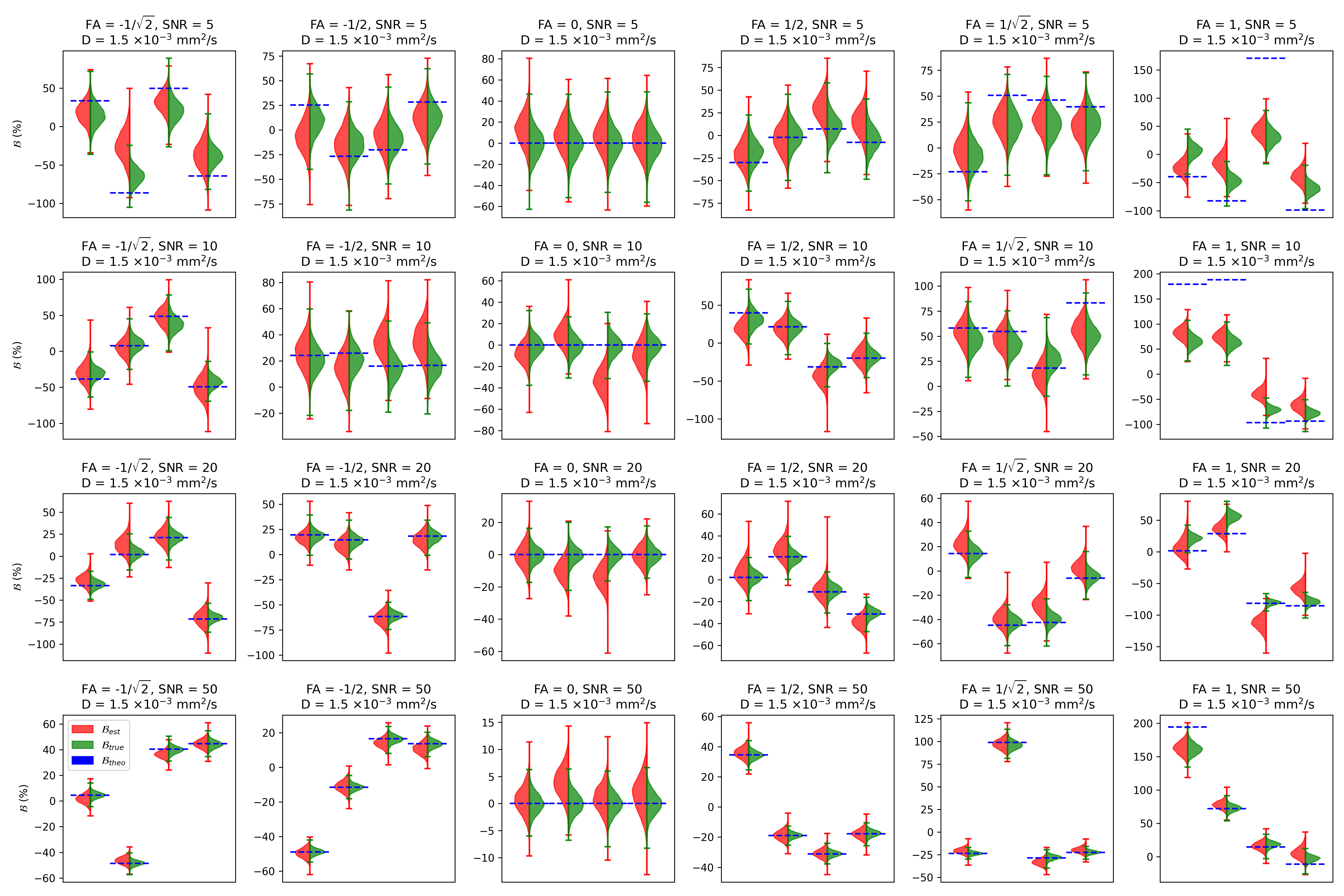
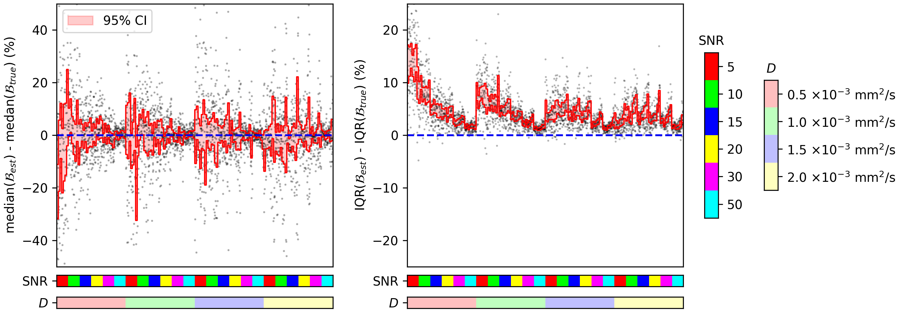
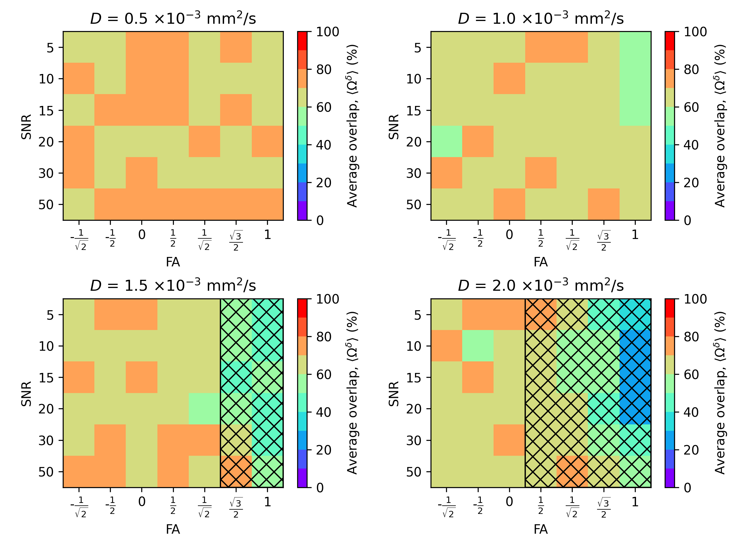
Figure 1 presents violin plots of $$$\mathcal{B}_{true}$$$ and $$$\mathcal{B}_{est}$$$ from a subset of parameters ($$$D$$$ fixed at 1.5$$$\times 10^{-3}$$$ mm$$$^{2}$$$/s). There is good visual agreement over the range of parameters simulated. This is confirmed by the large average overlap (Figure 3) and OSI (Figure 4) observed over all tested combinations of parameters. In addition, initial evidence suggests that there is no systemic error when estimating the bias using MCMC sampling, though the widths of the derived distributions are likely over-estimated due to the uncertainty in the underlying tissue parameters (Figure 2). Finally, in all physically relevant combinations of parameters, we observed no significant difference between the estimated bias and the theoretical bias (Figure 5), other than for low SNR. Inference time for 4000 MCMC samples was 9.4-48.8 seconds (personal CPU) per simulation.

Conclusion

Bayesian inference of ADC bias provides a potent methodology for predicting the discrepancy of measurements derived under different experimental conditions. This depends on availability of suitable data (MDDW in this case), but does offer the intrinsic uncertainty in all estimates. This could allow pixel-wise comparison of two measurement approaches without the need to directly acquire datasets, saving resources.

Acknowledgements

This project represents independent research funded by the National Institute for Health and Care Research (NIHR) Biomedical Research Centre at The Royal Marsden NHS Foundation Trust, The Institute of Cancer Research, London, the Royal Marsden Cancer Charity, London, The David and Ruth Lewis Family Trust and Sarcoma UK. The views expressed are those of the author(s) and not necessarily those of the NIHR or the Department of Health and Social Care.