INTRODUCTION

Morphologic changes of the bone are often found in knee osteoarthritis such as osteophyte formation. Bone fractures are also common. Bone imaging of the knee with MRI has been performed using sequences including ultrashort echo time (UTE),¹ and zero echo time (ZTE)² MRI. While promising, limitations of these techniques include low signal to noise and resolution. In this study, we describe and compare techniques to using a relatively new short-interval multiecho delta UTE (𝛅UTE)³ and multiecho 3D field echo (FE) acquisition (with and without high resolution deep learning reconstruction, DLR) followed by a simple post-processing that yields CT-like contrast.

METHODS

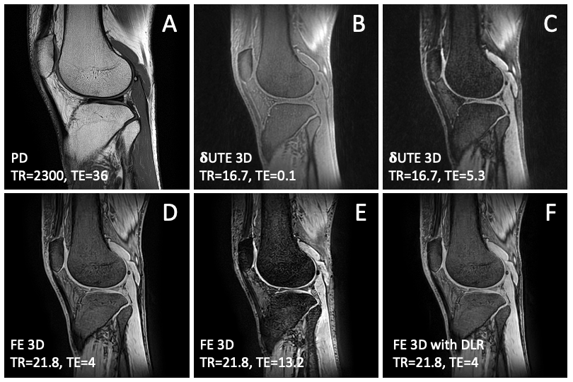
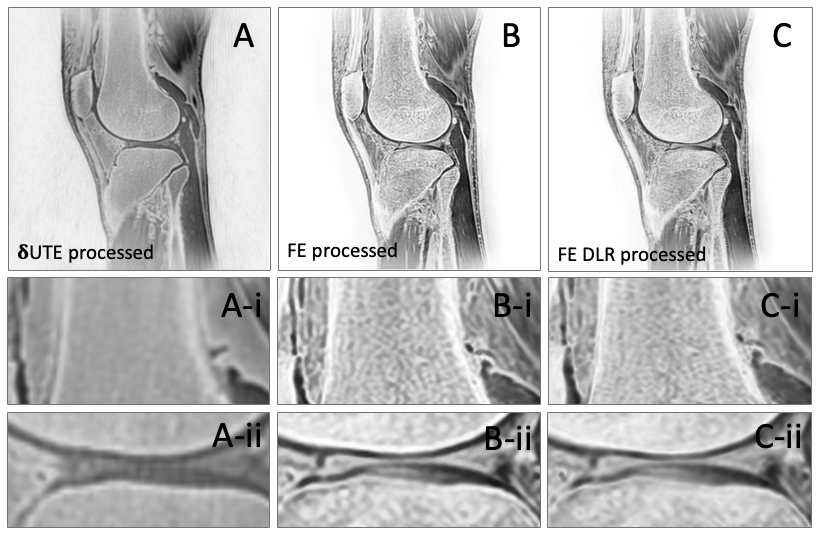
MRI: Right knees of four volunteers (n=4, 2 female, 32 ± 12.4 years old) were imaged at 3-T (Canon Galan) with a TR knee coil in the sagittal plane. One anatomical sequence and two bone-oriented sequences were used: (1) fast spin echo T2 weighted fat suppressed: TR=2300 ms, TE=36 ms, FOV=160 mm, matrix=448x448, slice=3 mm, ETL=7; (2) 3D 𝛅UTE multi-echo: TR=16.7 ms, TE=0.1, 0.5, 0.9, 1.3, 2.7, 5.3 ms, FOV=200 ms, matrix=256x256, slice=1 mm. (3) 3D field echo (FE) multi-echo: TR=21.8 ms, TE=4, 8.6, 13.2, 17.8 ms, FOV=200 mm, matrix=288x288, slice=1 mm. 4) high resolution deep learning reconstructed version of field echo (FE DLR): intensity corrected and super-resolution of the matrix to 864x864. The raw images are shown in Figure 1.
Image Processing: UTE, FE, and FE DLR images were processed by first averaging images from different TEs then inverting the averaged image. The processed images are shown in Figure 2.
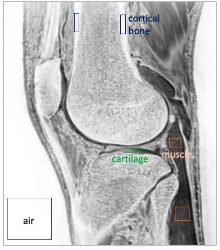
Signal-to-Noise Ratio (SNR), Contrast-to-Noise Ratio (CNR): Regions of interest (ROI) were drawn on a selected slice of the processed images through the lateral compartment of the knee for cortical bone, muscle, cartilage and the air (Figure 3) to determine SNR (mean signal intensity divided by standard deviation of noise in air) and CNR (difference in mean signal intensity between ROI divided by standard deviation of noise). Values were compared using ANOVA with posthoc Tukey test.
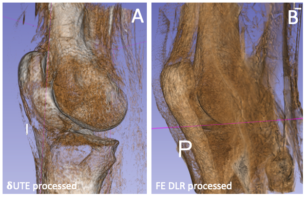
3D Rendering: On the processed images, bright background was segmented and inverted to low signal using region growing technique on ITK-SNAP. The resultant data was 3D rendered on Slicer 3D software.

RESULTS

Raw Images: Compared to conventional PD image (Figure 1A), 𝛅UTE images (Figure 1BC) depicted bone with low signal intensity and most other tissues with high signal intensity. FE images (Figure 1DE) also depicted bone with low signal but a few other tissues (ligaments and tendons) with low signal intensity. FE DLR (Figure 1F) provided a higher resolution, lower noise, and flatter intensity field compared to the raw FE image (Figure 1D).
CT-like Images: After processing, 𝛅UTE images (Figure 2A) had CT-like contrast, depicting cortical bone with high signal intensity (Figure 2A-i) but most other soft tissues with mid-to-low signal intensity. But 𝛅UTE processed image could not resolve trabecular bone (Figure 2A-ii). In contrast, both FE (Figure 2B) and FE DLR (Figure 2C) processed images depicted cortical and trabecular bone with high signal intensity. While FE and FE DLR images were overall similar, FE DLR appeared slightly sharper (Figure 2C-i) depicting cortical bone as thinner layer (Figure 2C-I and ii), while the FE image appeared more contrasty. This suggested that, due to high resolution, FE DLR could be useful for evaluating small bone injury such as hairline fracture, or changes in the trabecular bone, for example during osteoporosis.
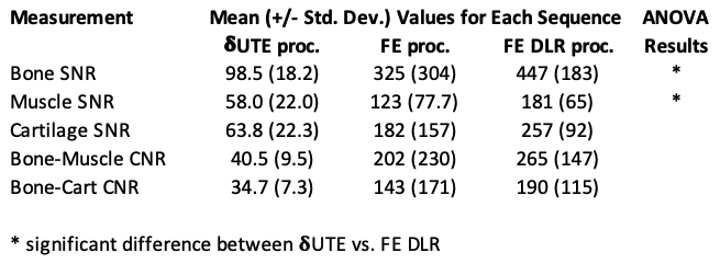
SNR, CNR: Table 1 summarizes SNR and CNR values for the processed CT-like images. While 𝛅UTE had good SNR ~100 and CNR ~40 for cortical bone, the values were generally greater when measured on FE and FE DLR. Bone SNR for FE DLR averaged over 400, with bone-muscle CNR over 200. There were significant (p<0.05) differences in Bone SNR between 𝛅UTE vs. FE DLR.
3D Render: Figure 4 shows 3D rendered images from 𝛅UTE (Figure 4A) and FE DLR (Figure 4B) data. While neither could perfectly segment bone based on intensity alone, 𝛅UTE fared somewhat better, unlike FE DLR rendering many non-bone tissues.

CONCLUSION

These results demonstrate the feasibility of bone MRI with CT-like contrast using existing sequences and simple image processing. Both 𝛅UTE and FE techniques provided good bone contrast, although FE DLR provide significantly greater bone SNR and depiction of fine trabecular bone structures. For 3D rendering of bone, UTE appeared better, as it provided better image contrast where the bone had the highest signal intensity that could be segmented via thresholding. While there is no MRI technique that provides a perfect CT-like contrast, continued advancement of MRI techniques may provide benefit for specific use cases.

Acknowledgements

Research reported in this publication was supported in part by a research grant from National Institute of Health (R01 AR066622 and P30 AR073761) in support of Dr. Bae, and a research grant support from Canon Medical Systems Corp., Japan (35938) in support of Dr. Miyazaki. The content is solely the responsibility of the authors and does not necessarily represent the official views of the sponsoring institutions.