5006
Nonlinear Susceptibility Inversion Deep Learning Model for Robust Quantitative Susceptibility Mapping1College of Electrical Engineering, Shenyang University of Technology, Shenyang, China, 2Neusoft Medical System, Shanghai, China
Synopsis
Keywords: Quantitative Imaging, Quantitative Susceptibility mapping, Susceptibility Inversion,Deep Learning
Motivation: Quantitative susceptibility mapping (QSM) estimates the spatial distribution of tissue susceptibility by solving a challenging ill-posed dipole inversion problem, which heavily affects the accuracy of tissue susceptibility quantification.
Goal(s): To generate high-quality QSM images.
Approach: In this study, we present a deep learning method for susceptibility inversion that utilizes a nonlinear susceptibility inversion model, NSIDL.Our approach integrated the Proximal Gradient Descent (PGD)[1] algorithm and embedding the physical model in the network.
Results: NSIDL was compared to traditional and deep learning methods, and it was found that NSIDL can effectively suppress streaking artifacts, mitigate noise amplification, and prevent excessive smoothing.
Impact: This study introduced the NSIDL deep learning method, which improved the accuracy of tissue magnetic sensitivity quantification. The improvement of QSM performance can help clinical doctors make more informed decisions based on reliable sensitivity measurements.
Introduction
Susceptibility inversion is the final and most critical step in the Quantitative Susceptibility Mapping (QSM) reconstruction process. It is an ill-posed inverse problem that heavily affect the precision of quantitative susceptibility measurements. Conventional QSM reconstruction methods often result in images with streaking artifacts, excessive smoothing, noise enhancement and underestimated magnetic susceptibility values. Data-driven deep learning-based methods frequently lack a data fidelity term in their network architecture, these models' predictions may deviate from the magnetic susceptibility values as determined by the dipole model on the original phase images. Therefore, we incorporate a nonlinear magnetic susceptibility inversion model into a deep learning network and utilize the PGD algorithm to systematically address the optimization problem. Taking the advantages of the nonlinear model and deep learning network, we obtain more precise estimates of susceptibility of the tissue.Methods
Theory The variational minimization problem for the ill-posed dipole inversion is given by:\hat{\chi}=argmin_{\chi}g\left(\chi\right)+R\left(\chi\right) (1)
Where g(\chi)=\frac{1}{2}\parallel D\chi-\phi\parallel_2^2, \chi is the magnetic susceptibility, \phi the local field, and R(\cdot) a regularizer. D is the dipole kernel, where D=F^{-1}DF applies the forward and inverse Fourier transform F.
According to nonlinear-MEDI[2], a nonlinear fidelity term can be used to optimize this formulation :
\hat{\chi}=argmin_{\chi}\parallel W\left(e^{iD\chi}-e^{i\phi}\right)\parallel_2^2+\parallel MG\chi\parallel_{1}(2)
Herein, the W serves as a data-weighting factor which can be the magnitude image or noise weight matrix. M is the anatomical prior and G is the gradient operator. This equation can be solved using a proximal gradient descent method:
\chi_{k}=Prox_{t_{k},R}\left(\chi_{k-1}-t_{k}\triangledown g\left(\chi_{k-1}\right)\right) (3)
Where Prox_{t_{k},R}\left(\cdot\right) is the proximity operator. The k^{th} update (iteration) of the reconstruction becomes:
\chi_{k}=Prox_{t_{k},R}\left(\chi_{k-1}-t_{k}D^{T}W^{T}Wsin\left(D\chi_{k-1}-\phi\right)\right) (4)
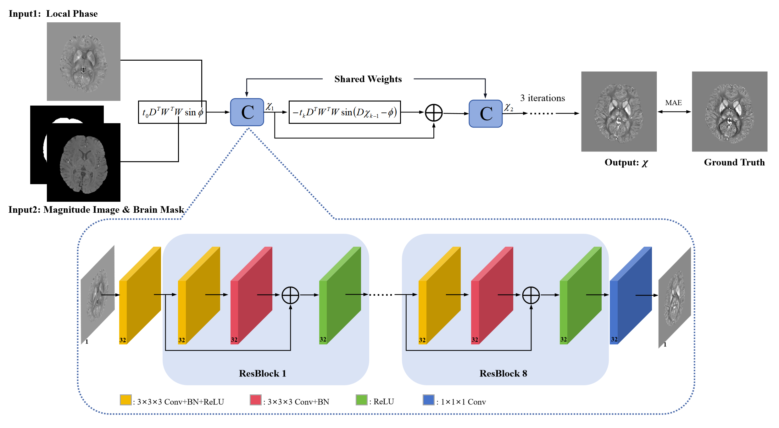
Where t_{k} is the step size in the k^{th} iteration in gradient descent.D^{T} is the conjugate transpose of D, the proximal operator Prox_{t_{k},R}\left(\cdot\right) only depends on R\left(\chi\right).Therefore, we can combine CNN with PGD to train a regularization term by learning its associated proximity operator, and replace Prox_{t_{k},R}\left(\cdot\right) with the learnable parameters,t_{k}.The iterates are initialized from \chi_{0}=0 and the input of the network is t_{0}D^{T}W^{T}Wsin\phi, and the final output is \chi_{k} which is given by the k^{th} iteration.
Network Architecture and Implementation Our network architecture is shown in Fig. 1. NSIDL is implemented in Tensorflow and trained on a NVIDIA GeForce RTX 2080 Ti GPU with mini-batch of size 2. To fit into GPU memory, the patch size for NSIDL training was cropped to 48 × 48 × 48. NSIDL was trained for 40 epochs, and the total training time was about 38 hours.
Data acquirement and processing Data was acquired from 8 healthy volunteers, for each volunteer, multiple head orientations were acquired, on a 3T scanner (Prisma, Siemens Healthineers, Erlangen, Germany), Data were acquired using a multi-echo 3D GRE sequence with the following parameters: FOV=210×224×160 mm3 , matrix size=210×224×160, flip angle=20°, bandwidth=190Hz/pixel,TR=44ms, TE=7.7/13.4/18.8/25.3/31.7/38.2ms, spatial resolution=1×1×1mm3,GRAPPA factor=2.[3]Laplacian unwrapping[4] and V‑SHARP[5] was performed. STI χ33 [6]was used as reference. In total, 144 groups of 3D local field maps and the corresponding labels from 8 subjects were obtained. Selected 90 groups of data from subjects 1-6, 80% of them were used for training and 20% for validation, and data from subjects 7-8 were used for testing.
Results
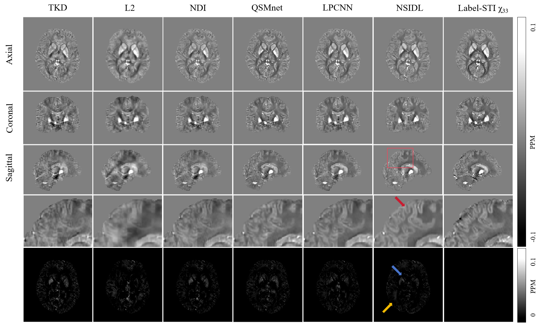
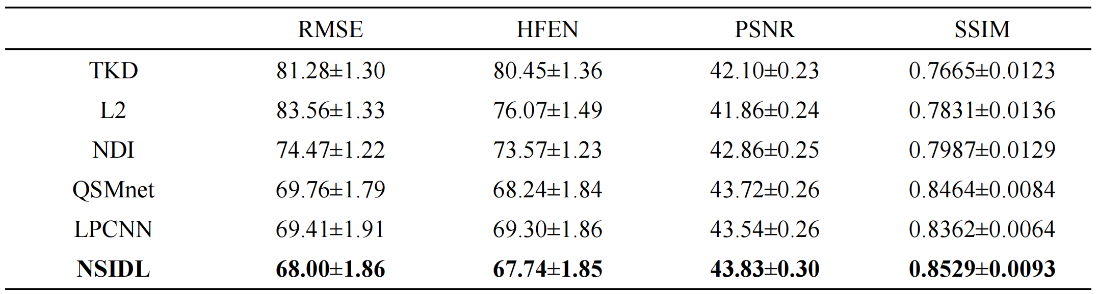
Fig.2 shows three orthogonal views of QSM maps and the difference maps relative to the label on one healthy subject using six QSM reconstruction methods(TKD[7],L2[8],NDI[9],QSMnet[10],LPCNN[11] and NSIDL). Table 1 shows the results of the six reconstruction methods evaluated by quantitative performance metrics of RMSE, HFEN, PSNR and SSIM.Discussion
As shown in Fig.2, the TKD reconstruction suffers from streaking artifacts, while L2 is over smoothing and NDI shows slight streaking effect.Compared to TKD, L2, NDI, and QSMnet, the LPCNN and NSIDL significantly reduced artifacts and noise,and our NSIDL showcases more high-frequency details.As pointed by the red arrows,a clear delineation between cortical gray matter and white matter was observed on NSIDL and the label maps. The blue arrow points to the caudate nucleus region in which TKD, NDI, QSMnet, and LPCNN exhibit significant divergence, and susceptibility values within the caudate nucleus were underestimated.The yellow arrow points to the cortical gray matter region,in which the NSIDL result shows minimum error when compared to other methods.The results in Table 1 show that NSIDL performs better than other methods in all criteria.Conclusion
In this work, we integrate a nonlinear susceptibility inversion model into a deep learning network to address the ill-posed dipole inversion problem in reconstructing MRI QSM image. The findings robustly establish that the NSIDL approach significantly capitalizes on the synergy between a nonlinear physical model and a 3D ResNet architecture to generate high-fidelity images suitable for precise quantification of tissue susceptibility.Acknowledgements
No acknowledgement found.References
[1] Parikh, N., & Boyd, S. (2014). Proximal algorithms. Foundations and trends® in Optimization, 1(3), 127-239.
[2] Liu, T., Wisnieff, C., Lou, M., Chen, W., Spincemaille, P., & Wang, Y. (2013). Nonlinear formulation of the magnetic field to source relationship for robust quantitative susceptibility mapping. Magnetic resonance in medicine, 69(2), 467-476.
[3] Shi, Y., Feng, R., Li, Z., Zhuang, J., Zhang, Y., & Wei, H. (2022). Towards in vivo ground truth susceptibility for single-orientation deep learning QSM: A multi-orientation gradient-echo MRI dataset. NeuroImage, 261, 119522.
[4] Schofield, M. A., & Zhu, Y. (2003). Fast phase unwrapping algorithm for interferometric applications. Optics letters, 28(14), 1194-1196.
[5] Wu, B., Li, W., Guidon, A., & Liu, C. (2012). Whole brain susceptibility mapping using compressed sensing. Magnetic resonance in medicine, 67(1), 137-147.
[6] Liu, C. (2010). Susceptibility tensor imaging. Magnetic Resonance in Medicine: An Official Journal of the International Society for Magnetic Resonance in Medicine, 63(6), 1471-1477.
[7] Shmueli, K., de Zwart, J. A., van Gelderen, P., Li, T. Q., Dodd, S. J., & Duyn, J. H. (2009). Magnetic susceptibility mapping of brain tissue in vivo using MRI phase data. Magnetic Resonance in Medicine: An Official Journal of the International Society for Magnetic Resonance in Medicine, 62(6), 1510-1522.
[8] Bilgic, B., Chatnuntawech, I., Fan, A. P., Setsompop, K., Cauley, S. F., Wald, L. L., & Adalsteinsson, E. (2014). Fast image reconstruction with L2‐regularization. Journal of magnetic resonance imaging, 40(1), 181-191.
[9] Polak, D., Chatnuntawech, I., Yoon, J., Iyer, S. S., Milovic, C., Lee, J., ... & Bilgic, B. (2020). Nonlinear dipole inversion (NDI) enables robust quantitative susceptibility mapping (QSM). NMR in Biomedicine, 33(12), e4271.
[10] Yoon, J., Gong, E., Chatnuntawech, I., Bilgic, B., Lee, J., Jung, W., ... & Lee, J. (2018). Quantitative susceptibility mapping using deep neural network: QSMnet. Neuroimage, 179, 199-206.
[11] Lai, K. W., Aggarwal, M., van Zijl, P., Li, X., & Sulam, J. (2020). Learned proximal networks for quantitative susceptibility mapping. In Medical Image Computing and Computer Assisted Intervention–MICCAI 2020: 23rd International Conference, Lima, Peru, October 4–8, 2020, Proceedings, Part II 23 (pp. 125-135). Springer International Publishing.
Figures