4686
A KomaMRI Phantom Extension for Integrated Dynamic Imaging1Laboratorio de Procesado de Imagen, Universidad de Valladolid, Valladolid, Spain, 2Department of Electrical Engineering, Pontificia Universidad Católica de Chile, Santiago, Chile, 3Dpto. de Ingeniería Energética y Fluidomecánica, Universidad de Valladolid, Valladolid, Spain
Synopsis
Keywords: Software Tools, Simulations, Motion modelling
Motivation: KomaMRI is a newly released Pulseq-compatible MRI simulator. Albeit the simulator includes dynamic imaging, motion type is limited to analytical expressions.
Goal(s): To provide KomaMRI with additional dynamic properties irrespective of the motion type.
Approach: To expand the phantom class to account for sampled arbitrary trajectories and to interpolate spin positions at time instants needed for the simulation. The simulation kernel is valid almost “as is” and only the demagnetization of the spins leaving the volume needs to be accounted for.
Results: 2D Cardiac cine with bright-blood effect, tagging and flow both with in-house and XCAT phantoms are dealt with now in KomaMRI.
Impact: KomaMRI is expected to be used for designing and testing novel pulse sequences. The added capabilities provided by the extension we propose increase its potential associated by enabling the simulator to deal with any sort of motion for sequence design.
Purpose
KomaMRI1, a Julia2 package that simulates the MRI process requires as input the definition of the phantom, the scanner and the sequence. The former contains information about each spin, namely, its initial position in the three axes and its magnetic properties (PD, T1 and T2). As for motion, it can be analytically defined using functions that are applied “on the fly” to all the spins in the volume. This method limits realistic motion simulation due to the difficulty of analytically defining realistic organ motion or flow models in closed-form expressions. Our purpose is to expand the phantom definition to accommodate realistic motion models in the simulator.Methods
To implement the phantom, we defined a new file format that extends its original definition. We also defined an interpolation mechanism, and slightly modified the simulation functions.Phantom class extension:
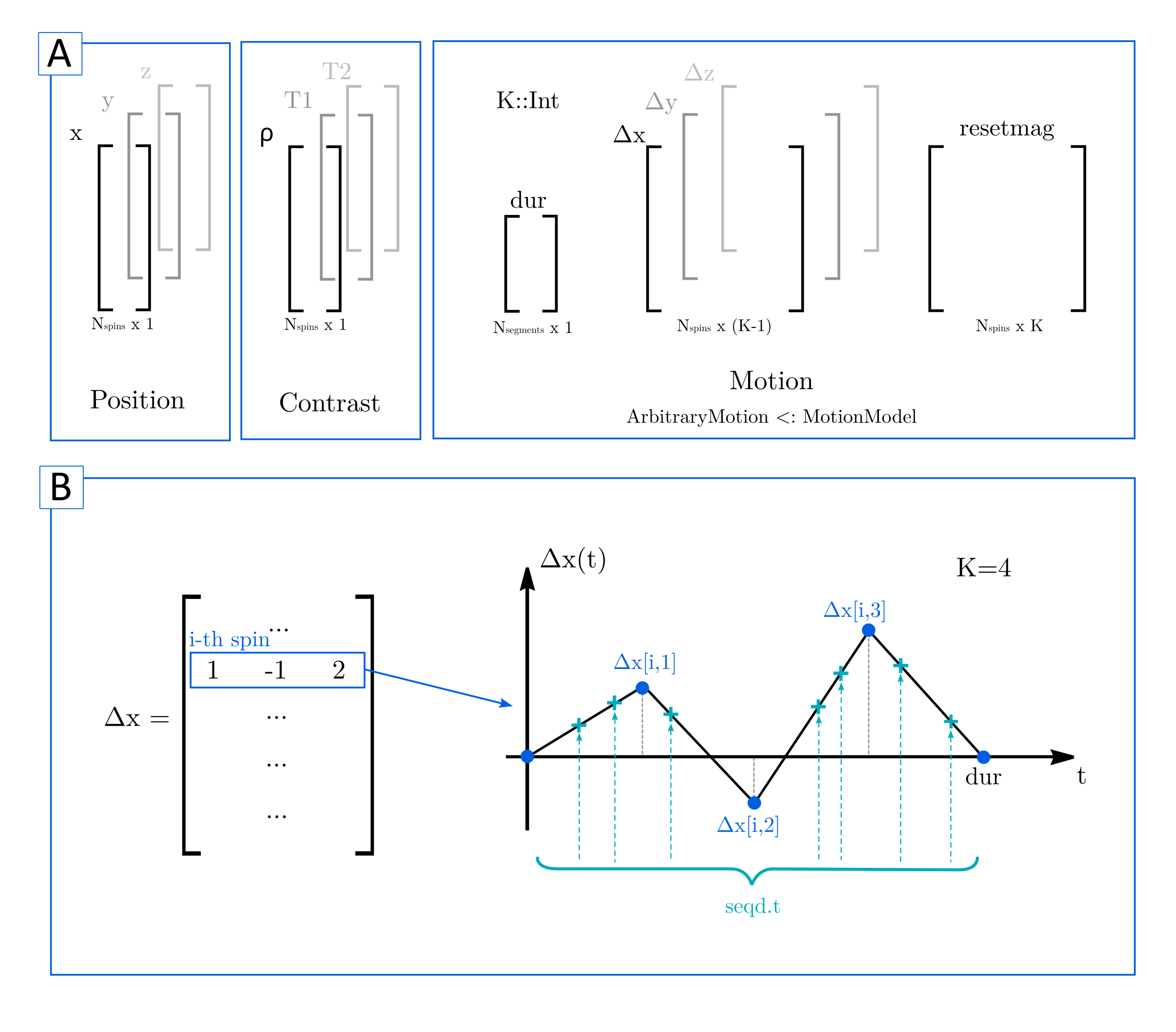
A new motion model, referred to as ArbitraryMotion, has been included in the phantom for which closed-form expressions are no longer needed. Motion can now be expressed as a list of spin positions in space. Figure 1A shows the phantom structure. Displacements are stored in matrices Δx, Δy and Δz, with each row corresponding to a spin and each column to a discrete time instant. For periodic motion, parameter dur stores the cycle duration. Pseudo-periodic motion (such as arrhythmias) is accounted for by letting this parameter be a vector with different components. Each cycle is divided in K pieces, as illustrated in Figure 1B. Matrix resetmag contains flags that indicate when a reset in the magnetization of a spin should be carried out. This is necessary for simulating inflow and outflow of spins.
Interpolation:
Figure 1B shows how spin position is determined for each time step of the simulation. A piecewise linear interpolation is carried out, considering the Δx values (and similarly for the other two dimensions) as nodes. Interpolation is carried out in parallel prior to the simulation, since time instants are known and determined by the sequence. This pre-computed positions, and their corresponding resetmag flags, are passed to the actual simulation functions.
Simulation functions:
The phantom definition suits the current code since dynamic positions of the spin can be precomputed. Hence, only the magnetization state of the spins leaving the phantom volume must be reset. This is a straightforward operation in Julia due to its vector indexing capabilities.
Results
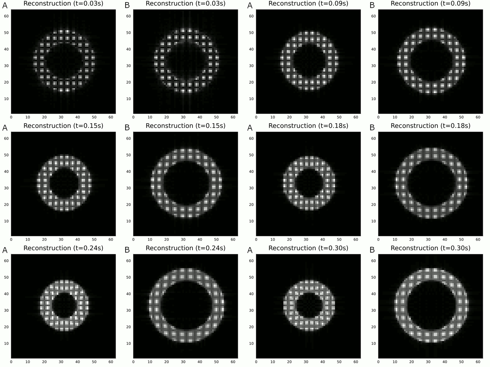
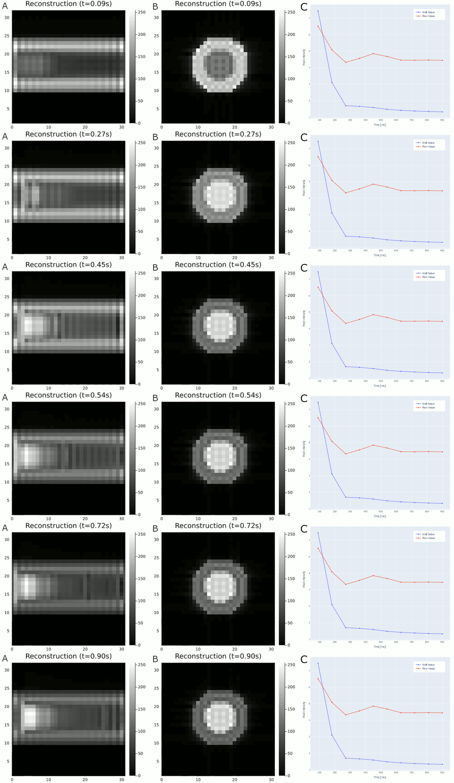
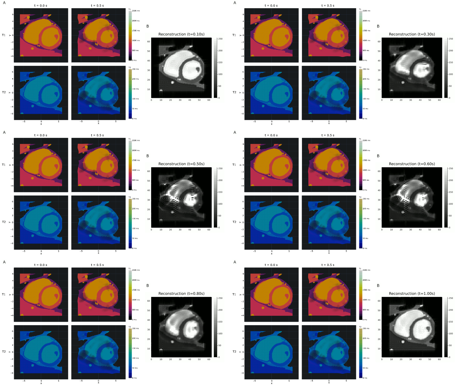
Figure 2 shows a tagging-like acquisition carried out with a BSSFP sequence on a phantom with motion trajectories defined by analytical expressions but treated as expected in the ArbitraryMotion model. Figure 3 shows a cylindrical phantom in which particles that simulate blood spins are injected on in the left-hand side of the cylinder and move rightwards. Figures 3A and 3B show, respectively, a longitudinal and an axial slice of the cylinder where 2D cine is simulated by means of the bSSFP sequence. Figure 3C shows the bright-blood effect encountered in 2D cine due to fresh blood particles entering the area where the steady state has already been reached by the spins on the myocardium. Finally, Figure 4 shows a cine image executed on an XCAT3 model where material point trajectories are expressed by a sequence of positions. Color images show the T1 (upper) and T2(lower) maps at end-diastole and end-systole (left and right respectively) and the image on the right-hand side shows the cine reconstruction.Discussion
KomaMRI indeed includes a dynamic model for phantom elastic motion; actually, the result in Figure 2 is obtainable with the original KomaMRI since spins motion is expressed by closed-form expressions. Other more involved motions per-se (Fig. 3) or motions obtained from external resources (such as XCAT) as a list of spatial positions (Fig. 4) require an extension such as the one we propose. We are aware of other simulators in which motion is also accounted for; one example is CMRSim4. The advantage of our model is that we have no difference in processing according to the type of motion we intend to simulate, since organ motion and flow (and, eventually diffusion) are handled similarly with minor changes in the simulation kernel functions. The downside of our approach is the amount of memory needed since, for the same number of spins, memory consumption increases to give room to the precalculated trajectories.Conclusion
KomaMRI has been extended to accommodate motion models for which an analytical closed form expression is not available. Future research will focus on improving the implementation of the model here proposed so that memory requirements are alleviated.Acknowledgements
The authors acknowledge grants PID2020-115339RB-I00, TED2021-130090B-I00 and PID2021-124407NB-I00 from the Ministerio de Ciencia e Innovación of Spain.References
- Castillo-Passi C, Coronado R, Varela-Mattatall G, Alberola-López C, Botnar R, Irarrazaval P. KomaMRI.jl: An open-source framework for general MRI simulations with GPU acceleration. Magn Reson Med. 2023; 1-14.
- Bezanson J, Edelman A, Karpinski S, Shah V.B, Julia: A fresh approach to numerical computing, SIAM review. 2017; 59(1): 65-98.
- Segars W.P, Sturgeon G, Mendonca S, Grimes J, Tsui B.M.W. 4D XCAT phantom for multimodality imaging research. Medical Physics. 2010; 37: 4902-4915.
- Weine J, McGrath C. CMRSim – A Python package for MRI simulations incorporating complex organ motion and flow. Cardiovascular Magnetic Resonance Imaging group at ETH Zurich. https://people.ee.ethz.ch/~jweine/cmrsim/latest/index.html Accesed November 8, 2023.
Figures