Introduction

There are many implementations for simulating the Bloch equations and their extensions^1-9. The high computational cost of the simulation was a common problem to be overcome. Several algorithms such as utilization of combined transitions^3-5 and no temporal changes⁶ were effective for reducing the computational cost. Special hardware such as general-purpose graphics processing unit (GPGPU)^6-8, and cloud computing⁹ was also effective. Nevertheless, the simulation with several million isochromats was still time-consuming. The goal of this research is further reduction of its computational cost.

Methods

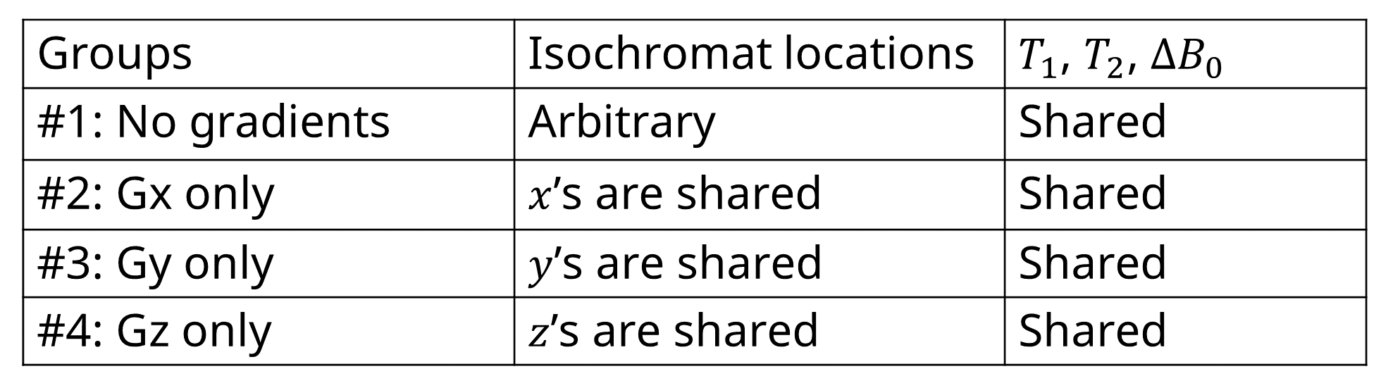
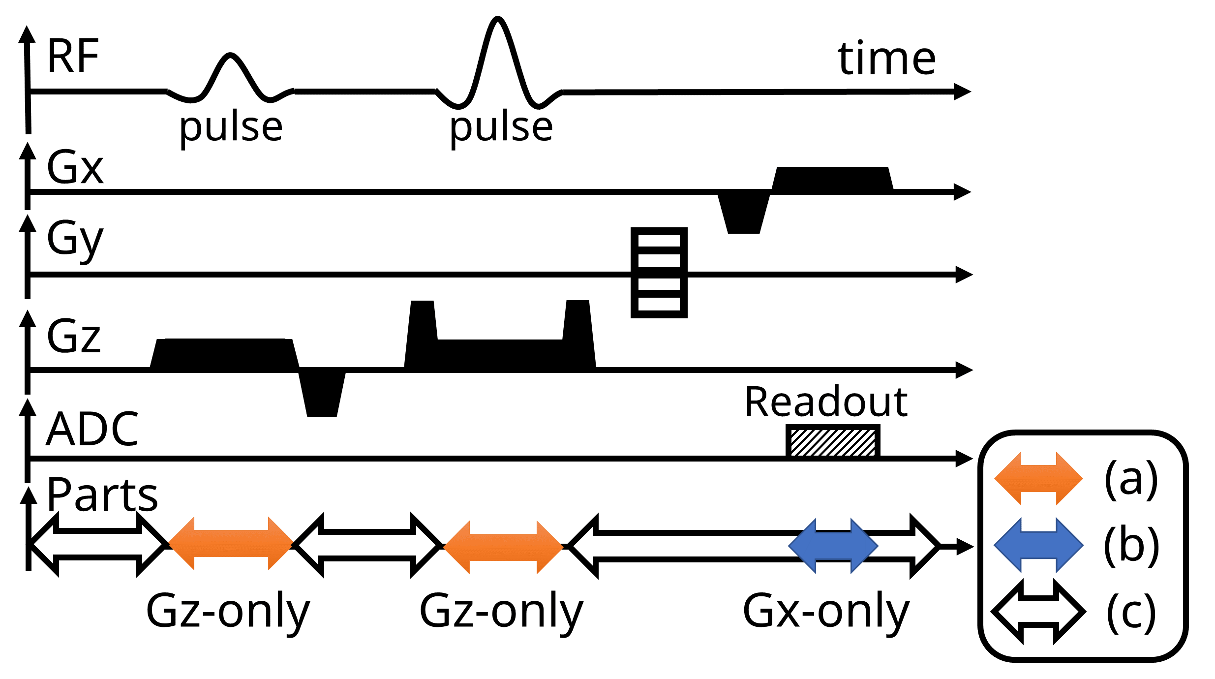
The author proposes a new computation method using grouped isochromats for further acceleration of the simulation. Before simulations, isochromats of a phantom were grouped for processing 4 different gradient types of sequences efficiently. The criteria used for grouping the isochromats are shown in Figure 1.
As shown in Figure 2, a pulse sequence to be processed was split into three parts: (a) with an RF pulse (with-RF), (b) with ADC sampling (with-ADC), and (c) other. The proposed method used a piecewise constant approximation (during $$$\Delta t=1$$$ microsecond) for processing a pulse sequence.
In processing with-RF and with-ADC parts, the proposed method tried to classify the part into one of the above-mentioned gradient types. If the classification was succeeded, grouped isochromats were combined for computing the processing part with the accelerated mode (explained later). Otherwise, the following conventional mode was used.
Conventional Mode
The with-RF part was processed by updating each magnetization $$$N_{RF}$$$ times. In an update step, the simulator multiplied a $$$4 \times 4$$$ transition matrix⁵ $$$\boldsymbol{U}(t,\Delta t,k)$$$ depending on RF pulse $$$B_{xy}(t)$$$, gradients $$$G_x(t)$$$, $$$G_y(t)$$$, and $$$G_z(t)$$$ of the with-RF part; and $$$T_1(k)$$$, $$$T_2(k)$$$, and $$$\Delta B_0(k)$$$ of the $$$k$$$-th isochromat. To compare with a state-of-the-art algorithm, the per-isochromat caching algorithm using combined transitions⁵ given as
$$U_{combined}(t_0,t_{N_{RF}},k)=\boldsymbol{U}(t_{N_{RF}-1},\Delta t,k)\cdots \boldsymbol{U}(t_0,\Delta t,k)$$
was also included in both conventional and acceleration modes.
In the with-ADC and other parts, magnetizations were updated from $$$t_0$$$ to $$$t$$$ by computing the analytic solution
$$M_{xy}(t,k)=M_{xy}(t_0,k)\exp \Big(-\frac{t-t_0}{T_2(k)}\Big)\exp \Big(\int_{t_0}^t -\gamma B_z(t,k) dt \Big),$$ and
$$M_z(t,k)=M_0(k) +(M_z(t_0,k)-M_0(k))\exp \Big(-\frac{t-t_0}{T_1(k)}\Big)$$
where $$$B_z(t,k)=G_x(t) x + G_y(t) y + G_z(t) z + \Delta B_0(k)$$$. In the with-ADC part, an ADC sample was given as $$$A(t)=\sum_k M_{xy}(t,k)$$$ when receiver coil sensitivities were not considered. When positions $$$(x,y,z)$$$ were not changed, these update required $$$N_{ADC}$$$ and 1 times for with-ADC and other parts, respectively.
For processing a phantom, the magnetizations of $$$K$$$ isochromats were updated for all three parts. The orders of the computation are $$$O(N_{RF}K)$$$, $$$O(N_{ADC}K)$$$, and $$$O(K)$$$ for with-RF, with-ADC and other parts, respectively.
Accelerated Mode
In the case of the with-RF part, isochromats in an isochromat group were designed for sharing properties for computing the above-mentioned transition matrix. Unlike the existing per-isochromat methods^3-5, the proposed method computed the above-mentioned combined transitions once, and multiplied $$$U_{combined}(t_0,t_{N_{RF}},k)$$$ to all isochromats for each isochromat group.
In the case of the with-ADC part, it was sufficient to compute the sum of magnetizations $$$\sum_k M_{xy}(t,k)$$$ for each isochromat group, and to compute $$$A(t)$$$ using the sums of magnetizations for all isochromat groups instead of magnetizations for all isochromats.
When number of isochromat groups $$$K_{group}$$$ is much less than $$$K$$$, the computational cost is reduced to $$$O(N_{RF}K_{group})$$$ and $$$O(N_{ADC}K_{group})$$$ for with-RF and with-ADC parts, respectively.
Evaluations
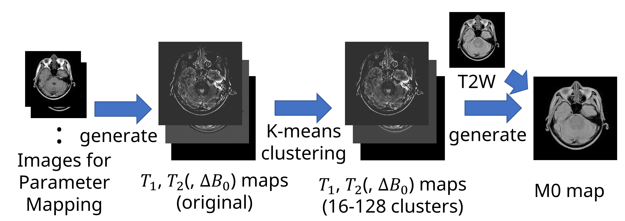
For running the proposed method efficiently, isochromats of a brain phantom (matrix size: $$$480 \times 480 \times 40$$$, FOV: $$$240 \times 240 \times 240$$$ mm³) were placed in grid points. The variations of isochromat parameters $$$T_1$$$, $$$T_2$$$ and $$$\Delta B_0$$$ were also limited to certain numbers using a k-means clustering method (with 16, 32, 64 and 128 clusters) for the accelerated mode, as shown in Figure 3.
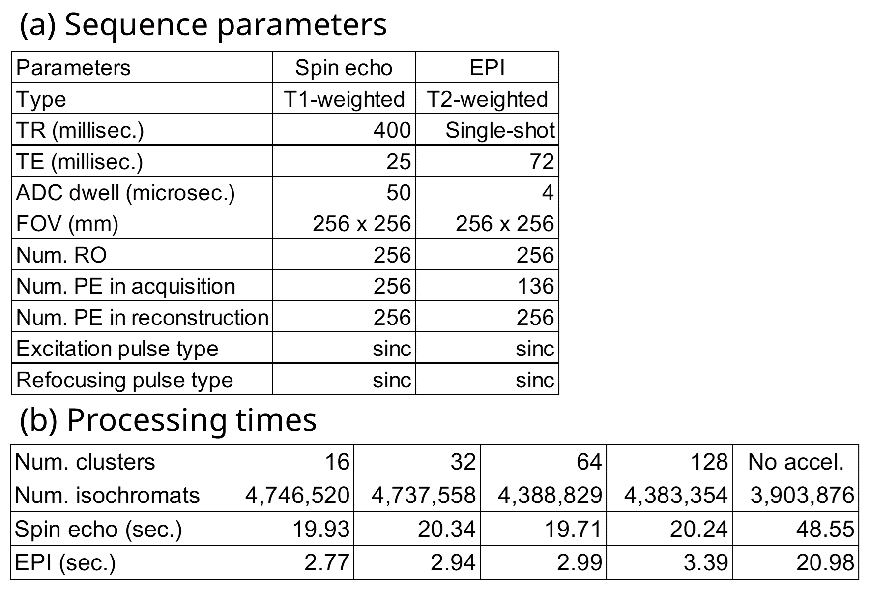
The processing time of single-slice spin-echo and EPI sequences (Figure 4 (a)) were evaluated with and without the accelerated mode of the proposed method.

Results

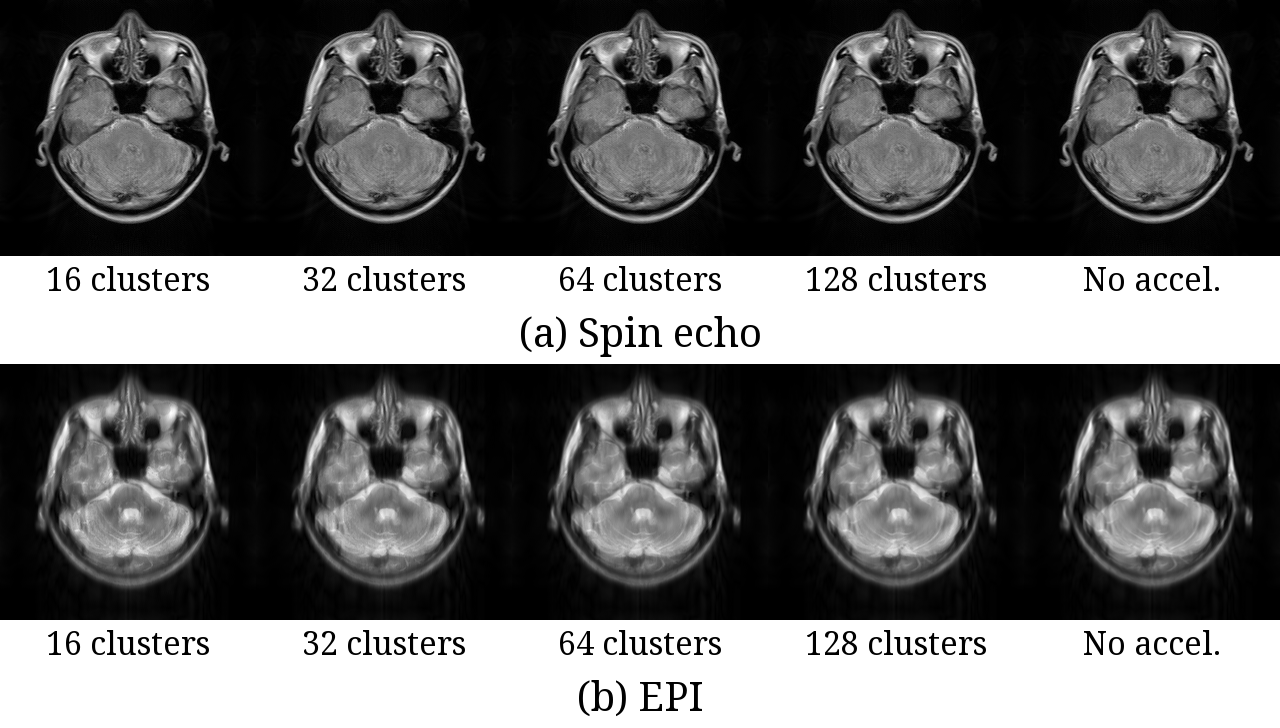
Individual processing time are shown in Figure 4 (b). Reconstructed images using a gridding algorithm for all cases are shown in Figure 5. The proposed method accelerated the simulation 2.4 and 6.2-7.7 times for spin-echo and EPI sequences, respectively.

Discussion

Processing grouped isochromats for individual parts of sequences reduced the computational cost of the simulation. Since there were no significant differences between the reconstructed images with and without clustering, using static isochromats pre-processed with a clustering algorithm was an efficient way for accelerating the simulation without losing reality of phantoms.

Conclusion

A new method using grouped isochromats was proposed for simulating the Bloch equations. The proposed method significantly reduced the computational cost without using special hardware for accelerating simulations.

Acknowledgements

The acquisitions of data used for generating the brain phantom were approved by our institutional review board and informed consent was obtained from the volunteer.