4655
Comparing k-space versus image domain loss functions in joint learning of sampling pattern and deep-learning reconstruction1Bernard and Irene Schwartz Center for Biomedical Imaging, Department of Radiology, New York University Grossman School of Medicine, New York, NY, United States, 2Center for Advanced Imaging Innovation and Research (CAI2R), Department of Radiology, New York University Grossman School of Medicine, New York, NY, United States
Synopsis
Keywords: Acquisition Methods, Machine Learning/Artificial Intelligence, Learned Sampling Patterns
Motivation: Joint learning of sampling pattern (SP) and deep-learning (DL) reconstruction can have their loss functions in the k-space or image domain. It is not clear which approach is better.
Goal(s): Investigate this question by comparing the results of both loss functions, exploiting the flexibility of k-space domain loss functions for joint learning.
Approach: We modify the training of DL reconstructions to compare image or k-space domain losses. We tested on two DL networks and two different datasets, always using raw k-space as input.
Results: The differences in image quality are very small, but there are visual differences in the learned SPs.
Impact: This investigation shows that image loss is also a good option, but k-space loss is more flexible to control the shape of the SP. Interestingly, different learned SPs, with slightly different distributions of k-space samples, led to similar quality results.
Introduction:
MRI can be accelerated by undersampling k-space data acquisition as long as undersampling artifacts are solved with special reconstructions (1–4), such as deep-learning (DL) reconstructions (3,5,6). More recently, new machine learning approaches were developed that allow for joint learning of the sampling pattern (SP) and the DL reconstruction (7–11), improving the quality and robustness of MRI.In this work, we investigate whether using the k-space domain loss function for joint learning of SP and the DL reconstruction is more effective than using the image domain loss function. We compared both approaches with two different DL reconstructions on two different datasets using the alternating learning, originally proposed in (10), with the stochastic bias-accelerated subset selection (SBASS) algorithm from (11). Here we show that k-space loss has some flexibility in controlling the shape of the learned SP.
Methods:
A DL reconstruction can be written as$$\hat{\mathbf{x}}=R_{\theta}(\mathbf{m}_Ω, Ω),$$
where $$$R_{\theta}$$$ represents the DL reconstruction with parameters $$$\theta$$$. We assume the following image-to-k-space model is used: $$$\mathbf{m}=\mathbf{FC}\mathbf{x}$$$, where $$$\mathbf{x}$$$ represents the 2D+time images, of size $$$N_x\times N_y \times N_t$$$ which denotes vertical $$$N_x$$$ and horizontal $$$N_y$$$ sizes and time $$$N_t$$$. $$$\mathbf{m}$$$ is the fully-sampled multi-coil k-t-space data. $$$\mathbf{C}$$$ denotes the coil sensitivities transform, estimated with (12), which maps $$$\mathbf{x}$$$ into multi-coil weighted images of size $$$N_x \times N_y \times N_t \times N_c$$$, with number of coils $$$N_c$$$. $$$\mathbf{F}$$$ represents the spatial FFTs, which are $$$N_t \times N_c$$$ repetitions of the 2D-FFT.
When undersampled is used, then $$$\mathbf{m}_{Ω}=\mathbf{S}_Ω\mathbf{FC}\mathbf{x},$$$ where $$$\mathbf{S}_Ω $$$ is the sampling function using SP $$$Ω$$$ (same for all coils). The SP contains $$$M$$$ k-t-space positions that will be sampled from a total of $$$N=N_x \times N_y \times N_t$$$ possible positions. The acceleration factor (AF) is defined as $$$N/M$$$.
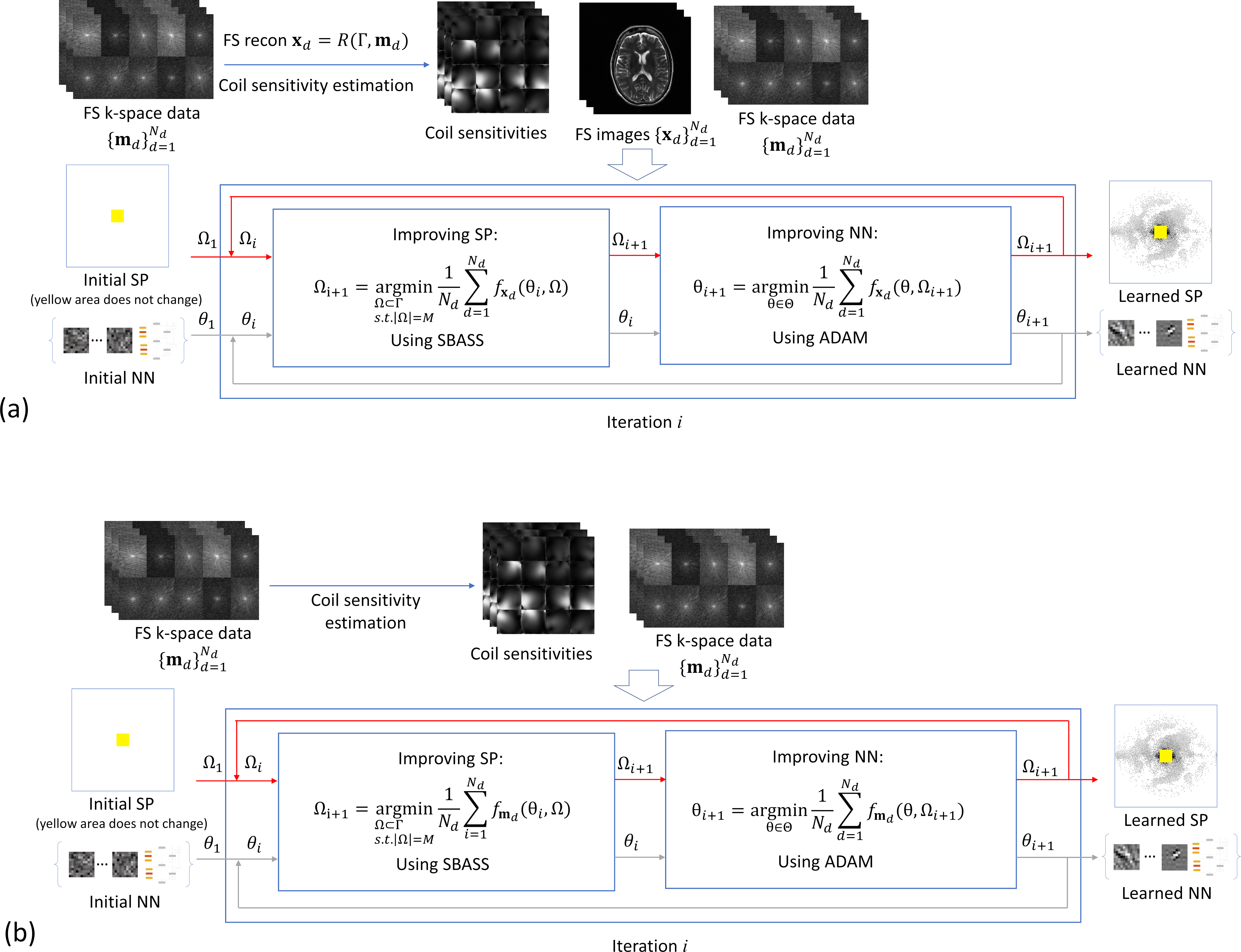
The alternating approach from (10), formulates the joint learning problem as
$$Ω_{i+1}=\arg\min_{\begin{array}{c}Ω \subset \Gamma\\ s.t. |Ω|=M\end{array}} \frac{1}{N_d} \sum_{d=1}^{N_d} f_d(\theta_i, Ω),$$
$$\theta_{i+1}=\arg\min_{\theta \in \Theta}\frac{1}{N_d}\sum_{d=1}^{N_d}f_d(\theta,Ω_{i+1}).$$
In the equations above, $$$N_d$$$ is the number of images used for training. In both cases, the minimization problem at each iteration is approximately solved with stochastic algorithms: ADAM (13) for DL and SBASS (11) for SP learning.
We used two DL reconstructions, one is a variational network (VN) (5), that represents a DL method with data-discrepancy layers (DDLs), and the other one is a simple UNET, with no DDLs, following implementations in (10). We modify the outputs of the networks to include an FS image-to-k-space transformation, so the loss function can be evaluated in the k-space, as shown in Figure 1. The loss $$$f_d(\theta,Ω)$$$ can be expressed in image domain as
$$f_{\mathbf{x}_d}(\theta,Ω)=||\mathbf{x}_d-R_{\theta}(\mathbf{m}_{d,Ω}, Ω)||^2_2,$$
where $$$\mathbf{x}_d=(\mathbf{FC})^+\mathbf{m}_d\approx\arg\min_{\mathbf{x}}||\mathbf{m}_d-\mathbf{FC}\mathbf{x}||^2_2$$$, is an FS reconstruction, while the weighted k-space loss is
$$f_{\mathbf{m}_d}(\theta,Ω)=||\mathbf{W}(\mathbf{m}_d-\mathbf{FC}R_{\theta}(\mathbf{m}_{d,Ω}, Ω))||^2_2,$$
In both cases, the input for reconstruction is the raw undersampled k-space data. We called VN-K and UNET-K the methods that use $$$\mathbf{W}$$$ as the identity, and VN-WK and UNET-WK when filter and weighting are used.
SBASS is guided by the measure of importance (MI), which plays an equivalent part of the gradient on differentiable problems, guiding the optimization. Typically, the MI used in SBASS (11) is constructed with
$$\mathbf{e}_d=\mathbf{FC}(\mathbf{x}_d-R_{\theta}(\mathbf{m}_{d,Ω}, Ω)),$$
when the loss is in the image domain. However, we also tested an MI in k-space, as
$$\mathbf{e}_d=\mathbf{W}(\mathbf{m}_d-\mathbf{FC}R_{\theta}(\mathbf{m}_{d,Ω}, Ω)),$$
Referred to as SBASS-K when $$$\mathbf{W}$$$ as the identity, and SBASS-WK otherwise. Here $$$\mathbf{W}$$$ increases the weights of high frequencies and filter noise in the null space of $$$\mathbf{FC}$$$.
We used two different datasets: 1) T2w Brain images (FastMRI dataset), size 320x320x1, training=450 images, validation=15 images, testing=15 images at acceleration factor (AF) of 12; and 2) T1rho knee joint images (our dataset), size 256x64x2, training=450 images, validation=15 images, testing=15 images at AF of 6.
Results:
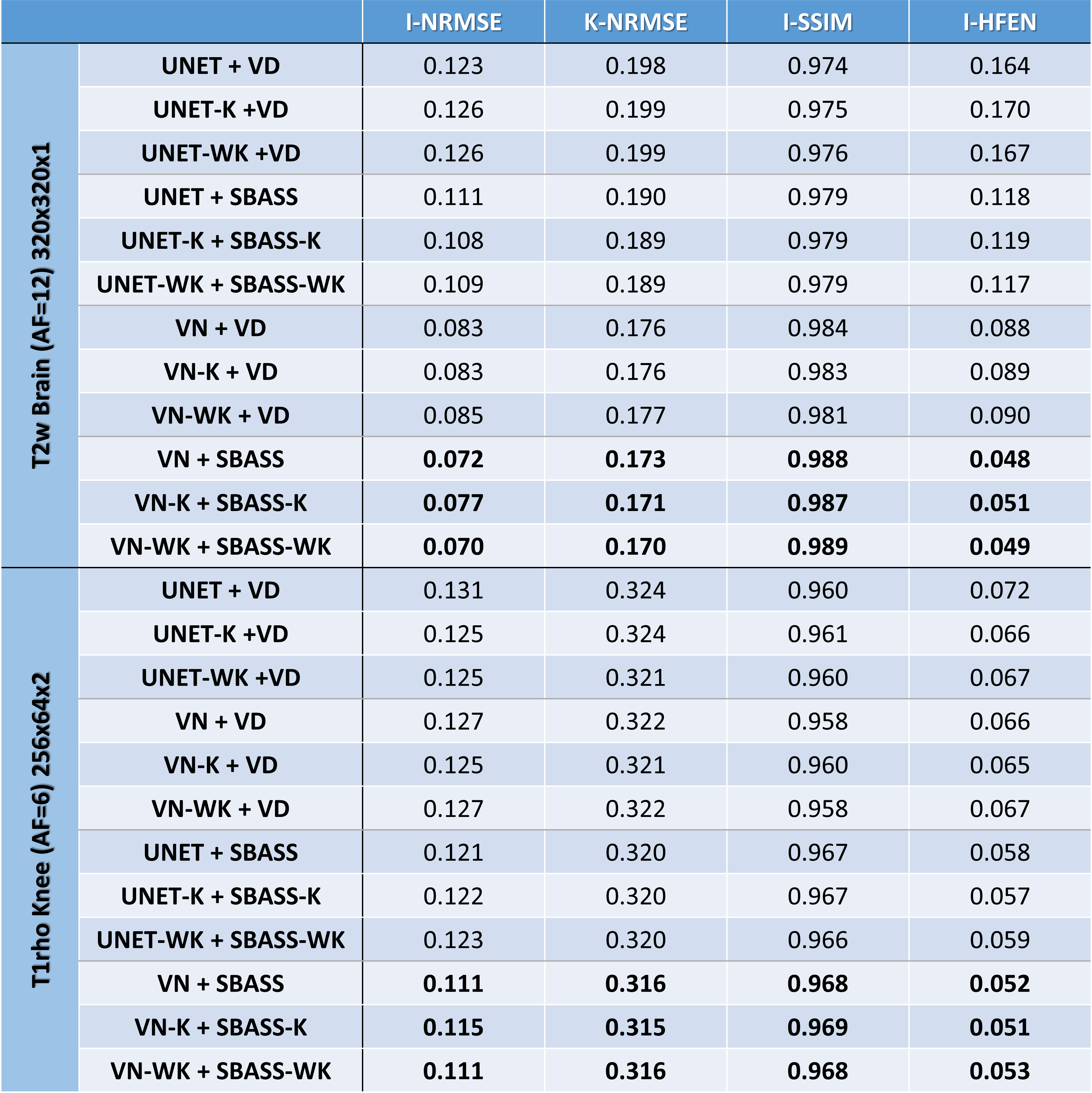
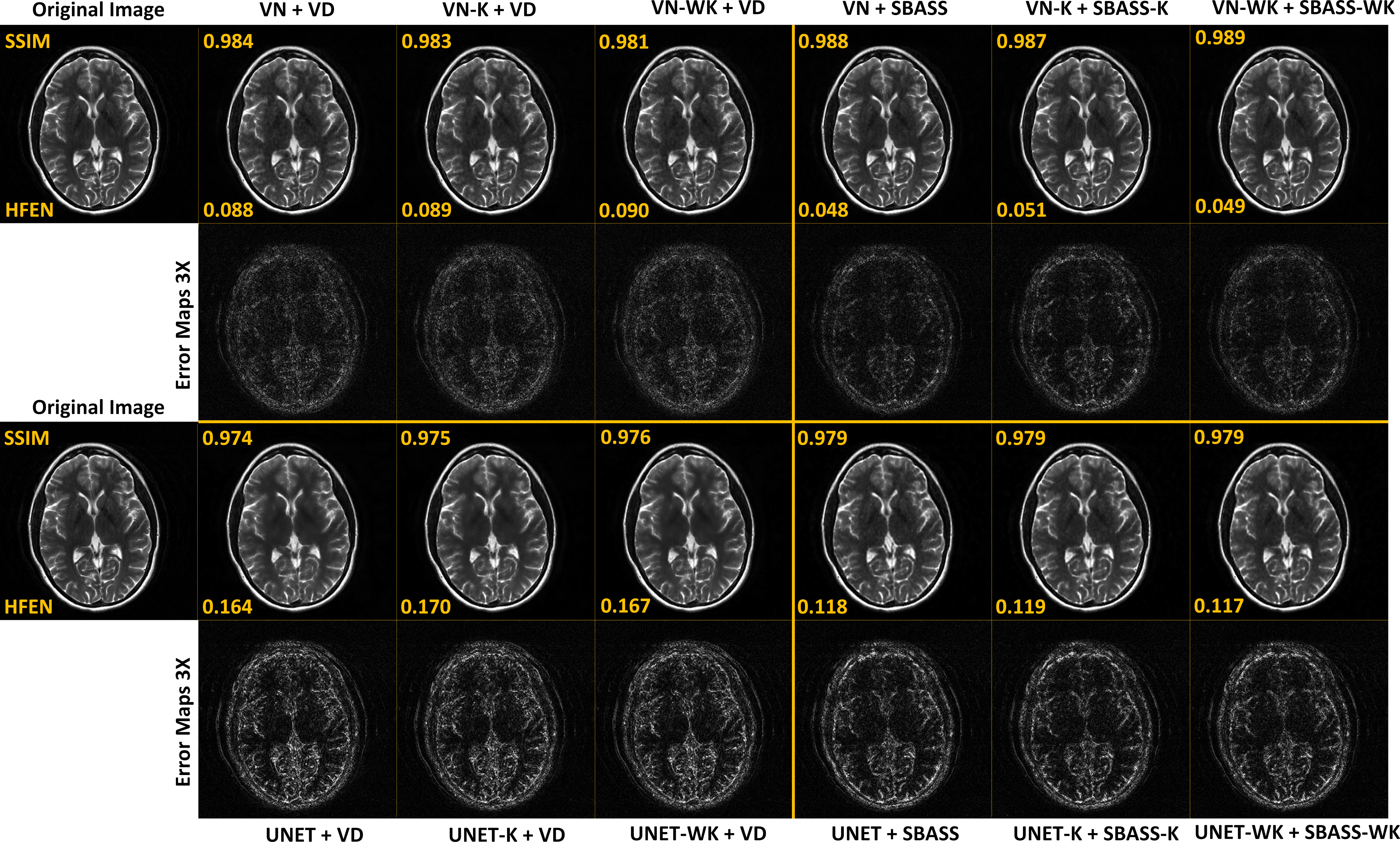
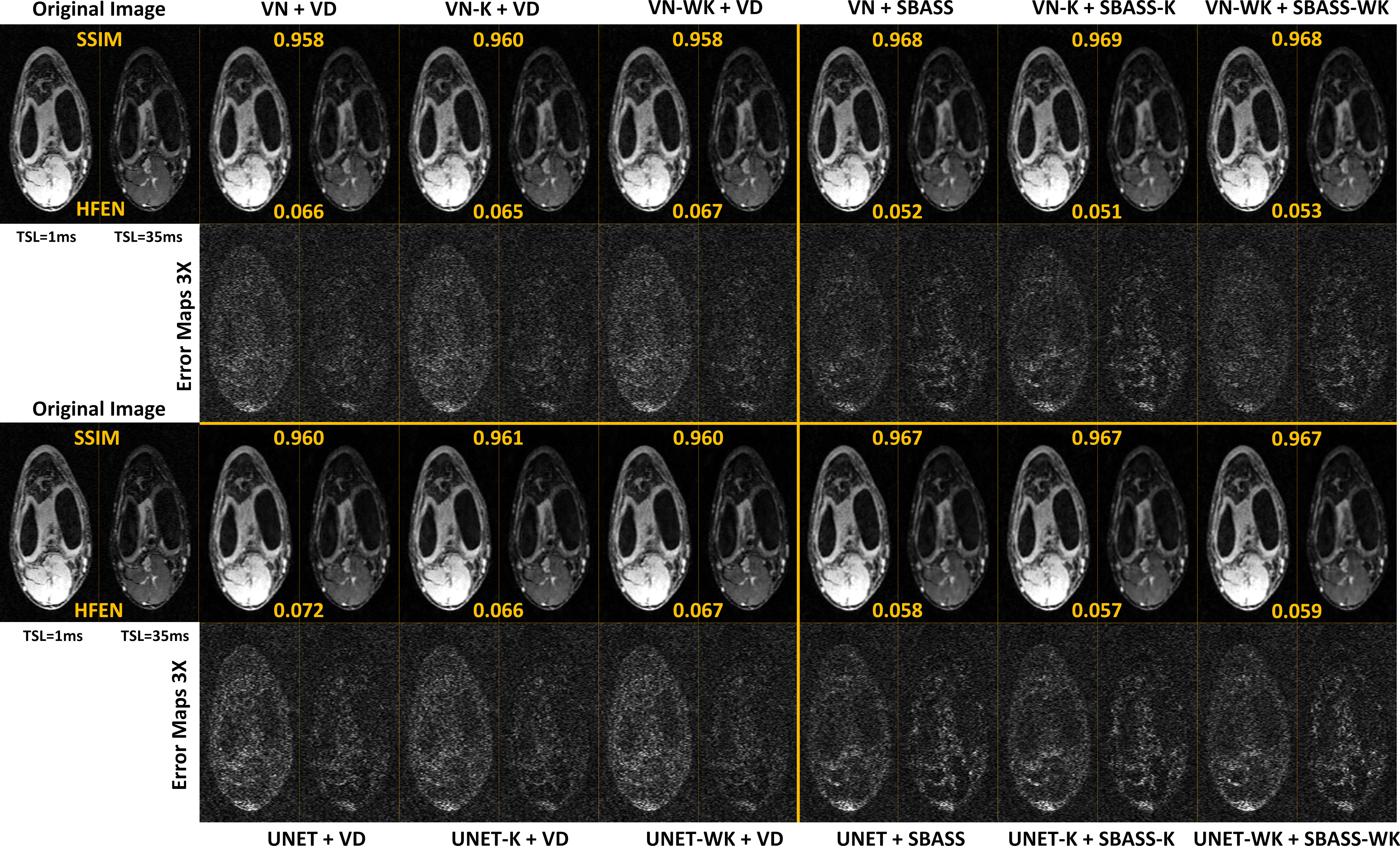
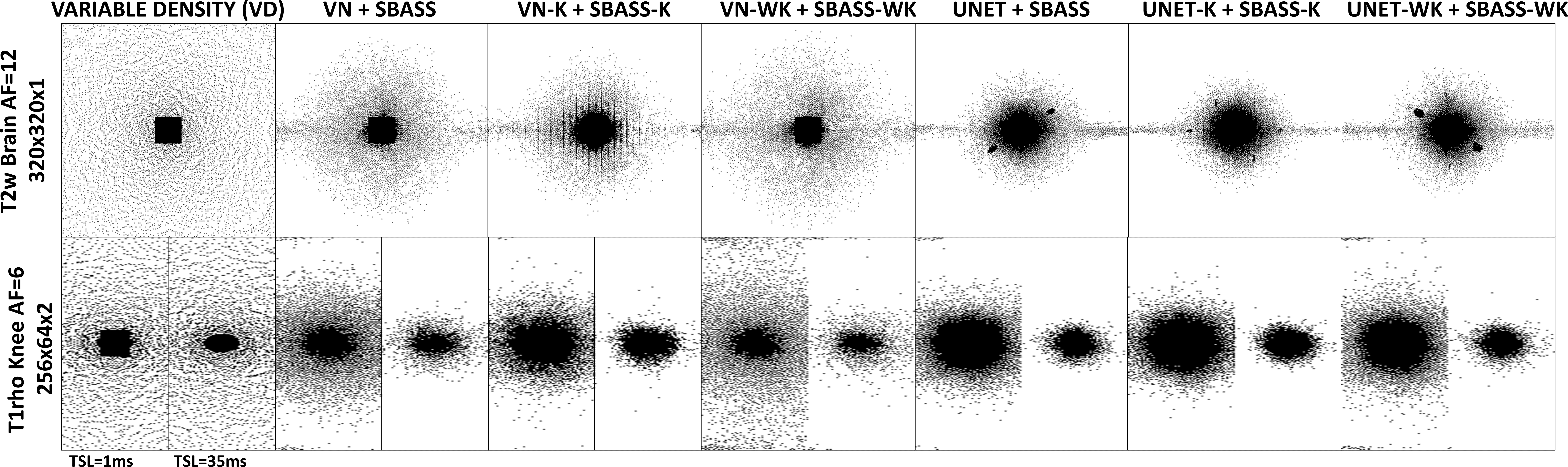
Table 1 shows numerical results with normalized root mean squared error (NRMSE) in the image domain (I-NRMSE) and k-space (K-NRMSE). We also show the SSIM (14) and HFEN (15). Some resulting images for T2w-brain and T1rho-knee datasets are shown in Figures 2, and 3 respectively. The learned SPs for both datasets are also shown in Figure 4.Discussion and Conclusion:
Loss in the k-space is potentially advantageous for joint learning, guiding the sampling distribution. However, we observe no significant advantages regarding the numerical values of quality (see Table 1 and Figures 2 and 3). However, as seen in Figure 4, the distribution of the k-space sampling is different, confirming that sampling density is not the only important property for efficient k-space sampling.Nevertheless, the use of SBASS, SBASS-K, or SBASS-WK in alternating learning once again demonstrated a significant improvement in image quality, being far superior to standard CS SPs such as VD.
Acknowledgements
This study was supported by NIH grantsR01-AR076328-01A1, R01-AR076985-01A1, and R01-AR078308-01A1 and was performed under the rubric of the Center of Advanced Imaging Innovation and Research (CAI2R), an NIBIB Biomedical Technology Resource Center (NIH P41-EB017183). Some Matlab codes for this work are available at https://cai2r.net/resources/combined-learning-of-accelerated-mri-sampling-and-reconstruction/References
1. Tamir JI, Ong F, Anand S, Karasan E, Wang K, Lustig M. Computational MRI With Physics-Based Constraints: Application to Multicontrast and Quantitative Imaging. IEEE Signal Process. Mag. 2020;37:94–104 doi: 10.1109/MSP.2019.2940062.
2. Feng L, Benkert T, Block KT, Sodickson DK, Otazo R, Chandarana H. Compressed sensing for body MRI. J. Magn. Reson. Imaging 2017;45:966–987 doi: 10.1002/jmri.25547.
3. Knoll F, Hammernik K, Zhang C, et al. Deep-learning methods for parallel magnetic resonance imaging reconstruction: A survey of the current approaches, trends, and issues. IEEE Signal Process. Mag. 2020;37:128–140 doi: 10.1109/MSP.2019.2950640.
4. Jacob M, Ye JC, Ying L, Doneva M. Computational MRI: Compressive Sensing and Beyond [From the Guest Editors]. IEEE Signal Process. Mag. 2020;37:21–23 doi: 10.1109/MSP.2019.2953993.
5. Hammernik K, Klatzer T, Kobler E, et al. Learning a variational network for reconstruction of accelerated MRI data. Magn. Reson. Med. 2018;79:3055–3071 doi: 10.1002/mrm.26977.
6. Liang D, Cheng J, Ke Z, Ying L. Deep magnetic resonance image reconstruction: Inverse problems meet neural networks. IEEE Signal Process. Mag. 2020;37:141–151 doi: 10.1109/MSP.2019.2950557.
7. Bahadir CD, Wang AQ, Dalca A V., Sabuncu MR. Deep-Learning-Based Optimization of the Under-Sampling Pattern in MRI. IEEE Trans. Comput. Imaging 2020;6:1139–1152 doi: 10.1109/TCI.2020.3006727.
8. Aggarwal HK, Jacob M. J-MoDL: Joint Model-Based Deep Learning for Optimized Sampling and Reconstruction. IEEE J. Sel. Top. Signal Process. 2020;14:1151–1162 doi: 10.1109/JSTSP.2020.3004094.
9. Weiss T, Vedula S, Senouf O, Michailovich O, Zibulevsky M, Bronstein A. Joint Learning of Cartesian under Sampling and Reconstruction for Accelerated MRI. In: IEEE International Conference on Acoustics, Speech and Signal Processing. Vol. 2020–May. IEEE; 2020. pp. 8653–8657. doi: 10.1109/ICASSP40776.2020.9054542.
10. Zibetti MVW, Knoll F, Regatte RR. Alternating Learning Approach for Variational Networks and Undersampling Pattern in Parallel MRI Applications. IEEE Trans. Comput. Imaging 2022;8:449–461 doi: 10.1109/TCI.2022.3176129.
11. Zibetti MVW, Regatte RR. Stochastic Bias-Accelerated Subset Selection Algorithm for Joint Learning of Sampling Pattern and Reconstruction in Accelerated MRI. In: IEEE International Symposium on Biomedical Imaging. IEEE; 2023. pp. 1–5. doi: 10.1109/ISBI53787.2023.10230762.
12. Uecker M, Lai P, Murphy MJ, et al. ESPIRiT-an eigenvalue approach to autocalibrating parallel MRI: Where SENSE meets GRAPPA. Magn. Reson. Med. 2014;71:990–1001 doi: 10.1002/mrm.24751. 13. Kingma DP, Ba J. Adam: A Method for Stochastic Optimization. arXiv Prepr. 2014:1–15.
14. Wang Z, Bovik AC, Sheikh HR, Simoncelli EP. Image quality assessment: from error visibility to structural similarity. IEEE Trans. Image Process. 2004;13:600–12.
15. Ravishankar S, Bresler Y. MR image reconstruction from highly undersampled k-space data by dictionary learning. IEEE Trans. Med. Imaging 2011;30:1028–1041 doi: 10.1109/TMI.2010.2090538.
Figures