4572
One-Step Image Reconstruction for Cine MRI with a Quadratic Constraint1Utah Valley University, Orem, UT, United States, 2University of Utah, Salt Lake City, UT, United States
Synopsis
Keywords: Image Reconstruction, Data Processing, dynamic imaging, closed-form solution, non-iterative methods
Motivation: In cine MRI, the measurements within each time-frame alone are too noisy for image reconstruction. Some information must be ‘borrowed’ from other time frames and the reconstruction algorithm is a slow iterative procedure.
Goal(s): We set up a constrained objective function, which uses the measurements at other time frames to regularize the image reconstruction. We derive a non-iterative algorithm to minimize this objective function.
Approach: The derivation of the algorithm is based on the calculus of variations. The resultant algorithm is in the form of filtered backprojection.
Results: The feasibility of the proposed algorithm is demonstrated with a clinical patient brain study.
Impact: Non-iterative reconstruction that minimizes a constrained objective function increases the throughput in healthcare institutions. This translates to reduced healthcare costs. The new reconstruction formula has a closed-form explicit expression of how to incorporate the reference image in dynamic reconstruction.
Introduction
Cine MRI provides detailed information on both anatomy changes and dynamic motion. It requires fast data acquisition, and the measurements may be noisy.Some image information changes fast from one time-frame to another, while some other image information changes slowly. Therefore, some image information can be ‘borrowed’ from neighboring time frames to assist image reconstruction at the current time.
Many methods are available to ‘borrow’ data outside of the current time frame. One popular method is the use of the low-rank constraint1-3. The low-rankness encourages the different images at different time frames to look like each other. An iterative algorithm is required to minimize the objective function, e.g., the alternating direction methods of multipliers (ADMM)4-5.
Some methods are based on the compressed-sensing framework6. They are solved by iterative algorithms; their associated objective functions commonly use the L1 or L0 norm.
This paper proposes an image-domain denoising method by ‘borrowing’ information from other time frames. The proposed algorithm is non-iterative with a closed-form formula. It is computationally efficient.
Methods
We consider the following objective function $$$v$$$ to be minimized:$$v(f)=||[Rf](s,\overrightarrow{\theta})-p(s,\overrightarrow{\theta})||^2 + \beta ||f-g||^2$$
where $$$f(\overrightarrow{x})$$$ is the 3D image to be reconstructed, $$$g(\overrightarrow{x})$$$ is a reference image that $$$f(\overrightarrow{x})$$$ should somewhat resemble, $$$RF$$$ is the 3D Radon transform of the function $$$f(\overrightarrow{x})$$$, $$$p(s,\overrightarrow{\theta})$$$ is a measurement of the Radon transform, and $$$\beta$$$ is a control parameter. The 3D Radon transform of the function $$$f(\overrightarrow{x})$$$ is7
$$[Rf](s,\hat{\theta}) = \iiint_\overrightarrow{x} f(\overrightarrow{x})\delta (\overrightarrow{x}\cdot \overrightarrow{\theta})d\overrightarrow{x}.$$
The method of the calculus of variations8 is used to find the optimal $$$f(\overrightarrow{x})$$$ by minimizing $$$v(f)$$$. The derivation starts with replacing the function $$$f(\overrightarrow{x})$$$ by the sum of two functions $$$f(\overrightarrow{x}) + \epsilon \eta (\overrightarrow{x})$$$.
The next step is to set the partial derivative of the objective function with respect to $$$\epsilon$$$ to zero. This leads to an Euler-Lagrange equation. The Euler-Lagrange equation in our case is
$$\iiint_\hat{x}f(\overrightarrow{x})[\frac{1}{||\hat{x}-\overrightarrow{x}||^2}+\beta \delta(\hat{x}-\overrightarrow{x} )]d\hat{x} = b(\overrightarrow{x})+ \beta g(\overrightarrow{x})$$
where $$$b(\overrightarrow{x})$$$ is the 3D Radon backprojection of the projection data $$$p(s,\overrightarrow{\theta})$$$ without filtering and is, in fact, the blurred version of the solution $$$f(\overrightarrow{x})$$$. The convolution kernel for this blurring effect is $$$\frac{1}{||\overrightarrow{x} ||^2}.$$$
The Fourier-domain counterpart of the above equation is given as
$$F(\overrightarrow{\omega})[\frac{1}{||\overrightarrow{\omega}||^2}+\beta]=B(\overrightarrow{\omega})+ \beta G(\overrightarrow{\omega})$$
and thus, we reach the final optimal solution in the closed form as
$$F(\overrightarrow{\omega}) = ||\overrightarrow{\omega}||^2 \frac{B(\overrightarrow{\omega}) + \beta G(\overrightarrow{\omega})}{1+ \beta ||\overrightarrow{\omega}|| ^2}.$$
This closed-form expression is the main result of our theoretical derivation. It shows that the optimal solution is a filtered version of the linear combination of the reference image and (surprise!) a blurred version of the unregularized reconstruction.
Discussion
Let us consider two extreme cases. When $$$\beta = 0$$$ (no regularization),$$F_{\beta = 0} (\overrightarrow{\omega}) = || \overrightarrow{\omega} ||^2 B(\overrightarrow{\omega}),$$
which is equivalent to the 3D Radon inversion formula. The Laplace operator in the Fourier domain is a filter represented by $$$|| \overrightarrow{\omega} ||^2 .$$$
If we change the order of filtering and backprojection, the filter becomes one-dimensional and is the second order derivative in the spatial (Radon) domain.
When $$$\beta \rightarrow \infty$$$ (too much regularization),
$$F_{\beta \rightarrow \infty}(\overrightarrow{\omega})=G(\overrightarrow{\omega}),$$
which is equivalent to $$$f = g$$$ in the spatial domain.
When $$$0< \beta <\infty$$$, we have a regularized reconstruction of $$$f$$$. The reference image $$$g$$$ can be chosen as the static image reconstructed by using the summation of all the measured k-space data from every time frames. It can also be chosen as the images reconstructed using a sliding time window. It can even be an image from other imaging modalities, such as x-ray CT after registration.
Results
A clinical patient brain study is presented here to illustrate the feasibility of the proposed method. The cine MRI data was acquired using a 3D golden angle radial trajectory. The k-space sampling looks like a koosh ball. Multiple coils were used in acquisition for parallel imaging, while only one coil was used for reconstruction in this paper. The reference image was chosen as the sum of the data from all time frames from one coil.Conclusions
Based on the 3D Radon inversion reconstruction and the calculus of variations, a constrained objective function is set up and optimized, resulting in a closed-form solution, in the form of filtered backprojection. This formula leads to a fast, non-iterative (one-step) algorithm. The proposed algorithm has a control parameter β. As illustrated by a dynamic clinical brain study, if this parameter is too large, the resulting reconstruction will look like the reference image. We must point out that the reconstructed image is not a weighted linear combination of an unconstrained reconstruction and the reference image.Acknowledgements
This work is supported in part by the NIH grants: RO1 NS 125635 and RO1 NS 127219.References
[1] Miao X, Lingala SG, Guo Y, Jao T, Usman M, Prieto C, Nayak KS. Accelerated cardiac cine MRI using locally low rank and finite difference constraints. Magn Reson Imaging. 2016 Jul;34(6):707-714. doi: 10.1016/j.mri.2016.03.007. Epub 2016 Mar 8. PMID: 26968142.
[2] Ke Z, Huang W, Cui ZX, Cheng J, Jia S, Wang H, Liu X, Zheng H, Ying L, Zhu Y, Liang D. Learned low-rank priors in dynamic MR imaging. IEEE Trans Med Imaging. 2021 Dec;40(12):3698-3710. doi: 10.1109/TMI.2021.3096218. Epub 2021 Nov 30. PMID: 34252024.
[3] Zonoobi D, Roohi SF, Kassim AA. Low-rank and sparse matrix decomposition with a-priori knowledge for dynamic 3D MRI reconstruction. Bioimaging (Bristol. Print) (2014).
[4] Boyd S, Parikh N, Chu EBP, Eckstein J. Distributed optimization and statistical learning via the alternating direction method of multipliers. Foundations and Trends in Machine Learning. 2011;3(1):1–122.
[5] Li J, Li J, Xie ,ZouJ, Plug-and-play ADMM for MRI reconstruction with convex nonconvex sparse regularization. IEEE Access, vol. 9, pp. 148315-148324, 2021, doi: 10.1109/ACCESS.2021.3124600.
[6] Lustig M, Donoho DL, Santos JM, Pauly JM. Compressed sensing MRI. IEEE Signal Processing Magazine, vol. 25, no. 2, pp. 72-82, March 2008, doi: 10.1109/MSP.2007.914728.
[7] Zeng GL. Medical Imaging Reconstruction, A Tutorial, ISBN: 978-3-642-05367-2, 978-7-04-020437-7, Higher Education Press, Springer, Beijing, 2009.
[8] Dacorogna B. Direct Methods in the Calculus of Variations. Springer-Verlag. ISBN 0-387-50491-5, 1989.
Figures
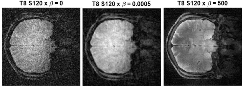
Reconstructed patient brain images at slice location of x = 120. Three different values of the control parameter β are used: 0, 0.0005, and 500.
When β = 0, no constraint is applied, and the image appears noisy.
When β = 500, the image appears the same as the reference image even though it is less noisy. This case should be avoided because this is not an accurate representation of the slice at time frame 8.
When β = 0.0005, the image is less noisy than the image without regularization and is a denoised version of it.
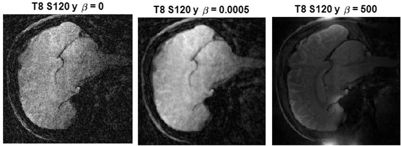
Reconstructed patient brain images at slice location of y = 120. Three different values of the control parameter β are used: 0, 0.0005, and 500.
When β = 0, no constraint is applied, and the image appears noisy.
When β = 500, the image appears the same as the reference image even though it is less noisy. This case should be avoided because this is not an accurate representation of the slice at time frame 8.
When β = 0.0005, the image is less noisy than the image without regularization and is a denoised version of it.
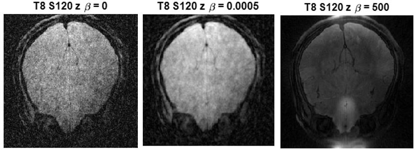
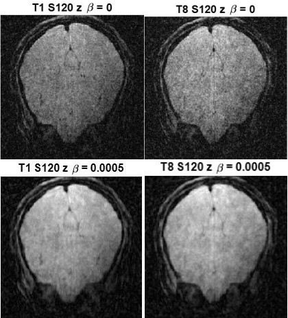
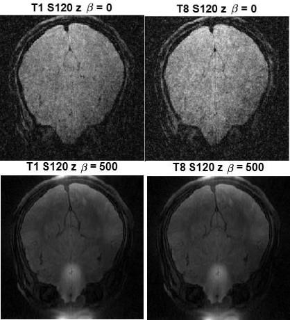
Reconstructed patient brain images at slice location of z = 120. Three different values of the control parameter β are used: 0, 0.0005, and 500.
When β = 0, no constraint is applied, and the image appears noisy.
When β = 500, the image appears the same as the reference image even though it is less noisy. This case should be avoided because this is not an accurate representation of the slice at time frame 8.
When β = 0.0005, the image is less noisy than the image without regularization and is a denoised version of it.