Introduction

In the past, accelerated MR quantitative T1ρ imaging was performed mainly through compressed sensing methods^1,2. Recently, deep-learning methods have been developed with promising performance^3,4. Most learning methods are based on the convolutional neural network(CNN) with U-net. These networks have to be trained to the specific subsampling scheme and are not generalized well to different subsampling patterns. More recently, denoising diffusion probabilistic models(DDPM) have been used to improve the performance of image reconstruction^5,6,7,8. The training of DDPM is independent of the sampling patterns so it has excellent generalization capabilities. In this study, we investigate the use of DDPM to accelerate T1ρ imaging, where the model is trained only for fully sampled data without the knowledge of subsampling patterns. The experiment shows DDPM improves over both the STFD⁹ and U-net¹⁰ when the subsampling patterns are different between training and testing, which generates the T1ρ map by reconstructing multiple T1ρ-weighted images with different spin-lock times(TSLs).

Method

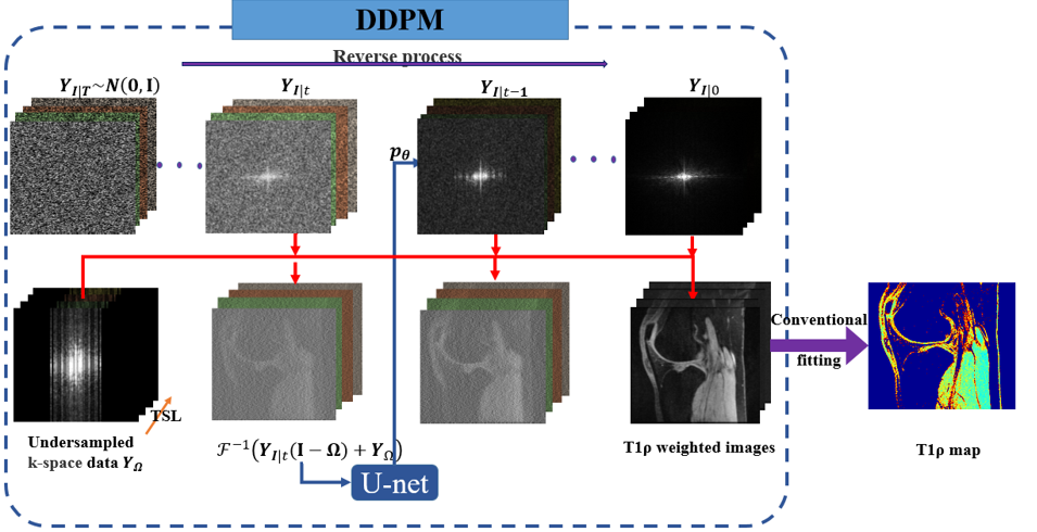
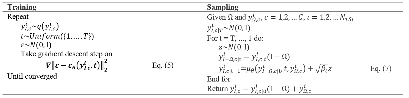
We perform DDPM on the subsampled k-space data $$$\bf Y_{\Omega}$$$ in Fig1. We defined $$$y_{\Omega,c}^i={\Omega}y_{I,c}^i$$$ and $$$y_{I-\Omega,c}^i=({I-\Omega})y_{I,c}^i$$$ as sampled and non-sampled k-space data, respectively, for each channel $$$c=1,2,...C$$$ with sampling pattern $$$\Omega$$$ and TSL $$$i=1,...N_{TSL}$$$, where $$$N_{TSL}$$$ is the total number of TSLs. $$$y_{I,c}^i$$$ is the full k-space data of channel $$$c$$$ and TSL $$$i$$$. The DDPM in k-space⁸ is used here, instead of the typical image-domain DDPM. We reconstruct each $$$y_{I,c}^i$$$ with data distribution of $$$y_{I,c}^i\sim{q(y_{I,c}^i\mid{y_{\Omega,c}^i})}$$$ only based on the non-sampled location $$$I-\Omega$$$ and sampled k-space measurements $$$y_{\Omega,c}^i$$$ using DDPM.
DDPM would be able to recover the information from the noise if we could learn the systematic decay process due to noise. Total two processes, diffusion, and reverse, in DDPM. In the diffusion process, we define a forward diffusion process in which Gaussian noise is successively added using a Markov chain according to $$$\beta_{1}<\beta_{2}...<\beta_{T}$$$ of the density function for T timesteps. The conditional probability density $$$q(y_{I,c\mid{t}}^i\mid{y_{I,c\mid{t-1}}^i})$$$ at a particular time t is parameterized as $$$N$$$:$$q(y_{I,c\mid{t}}^i\mid{y_{I,c\mid{t-1}}^i}):=N(y_{I,c\mid{t}}^i;\sqrt{1-\beta}y_{I,c\mid{t-1}}^i,\beta_{t}I)(1)$$ The distribution of entire forward process is:$$q(y_{I,c\mid{1:T}}^i\mid{y_{I,c\mid{0}}^i}):=\prod_{t=1}^Tq(y_{I,c\mid{t}}^i\mid{y_{I,c\mid{t-1}}^i})(2)$$ Set $$$\alpha_{t}+\beta_{t}=1,{\overline{a}}_{t}=\prod_{i=1}^t\alpha_{i}, \epsilon\sim{N(0,I)}$$$, we can sample $$$y_{I,c\mid{t}}^i$$$ at any timestep t:$$q(y_{I,c\mid{t}}^i\mid{y_{I,c\mid{0}}^i}):=N(y_{I,c\mid{0}}^i;\sqrt{{\overline{a}}_{t}}y_{I,c\mid{0}}^i,(1-{\overline{a}}_{t})I), y_{I,c\mid{t}}^i=\sqrt{{\overline{a}}_{t}}y_{I,c\mid{0}}^i+(1-{\overline{a}}_{t})\epsilon.(3)$$ Given a sufficiently large T, the latent $$$ y_{I,c\mid{T}}^i$$$ is nearly an isotropic Gaussian distribution. Thus, we can sample $$$y_{I,c\mid{T}}^i\sim{N(0,I)}$$$ and run the process in reverse to get $$$y_{I,c\mid{0}}^i$$$ if we know the exact reverse distribution $$$q(y_{I,c\mid{t-1}}^i\mid{y_{I,c\mid{t}}^i},y_{\Omega,c}^i)$$$ conditioned on $$$y_{\Omega,c}^i$$$ . We approximate the reverse distribution as: $$p_{\theta}(y_{I,c\mid{t-1}}^i\mid{y_{I,c\mid{t}}^i},y_{\Omega,c}^i):=N(y_{I,c\mid{t-1}}^i;\mu_{\theta}(y_{I-\Omega,c\mid{t}}^i,t,y_{\Omega,c}^i),\Sigma_\theta(y_{I-\Omega,c\mid{t}}^i,t,y_{\Omega,c}^i))(4),$$ where the mean and variance of Gaussian $$$N$$$ is: $$\mu_{\theta}(y_{I-\Omega,c\mid{t}}^i,t,y_{\Omega,c}^i)=\frac{1}{\sqrt{\alpha_{t}}}(y_{I,c\mid{t}}^i-\frac{\beta_{t}}{\sqrt{1-\overline{\alpha}_{t}}}\epsilon_{\theta}(y_{I-\Omega,c\mid{t}}^i,t,y_{\Omega,c}^i)),\Sigma_\theta(y_{I-\Omega,c\mid{t}}^i,t,y_{\Omega,c}^i)=\beta_{t}I,$$ and $$\epsilon_{\theta}(y_{I-\Omega,c\mid{t}}^i,t,y_{\Omega,c}^i)=F(D(F^{-1}(y_{I-\Omega,c\mid{t}}^i+y_{\Omega,c}^i),t;\theta))$$is the output of a U-net with $$$\theta$$$ being the parameters to learn, $$$F$$$ is the Fourier operator, and $$$D$$$ is the network to be trained by minimizing the following loss function:$$\theta^{*}=argmin_{\theta}{\parallel\epsilon-\epsilon_{\theta}(y_{I,c\mid{t}}^i,t)\parallel}_2^2,\epsilon_{\theta}(y_{I,c\mid{t}}^i,t)=F(D(F^{-1}(y_{I,c\mid{t}}^i),t;\theta))(5)$$ The complete distribution of the whole reverse process can then be computed as:$$p_{\theta}(y_{I,c\mid{0}}^i\mid{y_{I,c\mid{T}}^i},y_{\Omega,c}^i):=p_{\theta}({y_{I,c\mid{T}}^i},y_{\Omega,c}^i)\prod_{t=1}^Tp_{\theta}(y_{I,c\mid{t-1}}^i\mid{y_{I,c\mid{t}}^i},y_{\Omega,c}^i).(6)$$ We compute $$$y_{I,c\mid{t-1}}^i=\mu_{\theta}(y_{I-\Omega,c\mid{t}}^i,t,y_{\Omega,c}^i)+\sqrt{\Sigma_{\theta}(y_{I-\Omega,c\mid{t}}^i,t,y_{\Omega,c}^i)}(7)$$$ individually in table1, where $$$y_{I-\Omega,c\mid{t}}^i=y_{I,c\mid{t}}^i(I-\Omega).$$$ After the non-sampled data $$$\bf Y_{I-\Omega\mid{0}}$$$ for all channels are estimated, the T1ρ-weighted images $$$F^{-1}(\bf Y_{I-\Omega\mid{0}}+\bf Y_{\Omega})$$$ from all channels are obtained. Finally, conventional fitting is performed to obtain the T1ρ map.

Results and Discussion

Four sets of knee data were collected at a 3T GE scanner with 18 coils, using a magnetization-prepared angle-modulated partitioned k-space spoiled gradient echo snapshots(MAPSS) T1ρ(time of spin-lock[TSLs] of 0, 8, 24, 56ms, spin-lock frequency 500Hz, matrix size 384×192×60×4×18[FE×PE×Slice×Echo×Coil], FOV 14cm).
For all 4 TSLs and 60 slices, we cropped and zero-padded complex-valued 18-coil k-space data to 320×320(phase- and frequency-encoding directions). The center slices of three fully sampled sets(720 complex-valued multi-coil images) were used to train the networks and the rest set for testing. The testing data was retrospectively undersampled with 1D random patterns with reduction factors(4,6,8). Different sampling patterns are used for different TSLs.
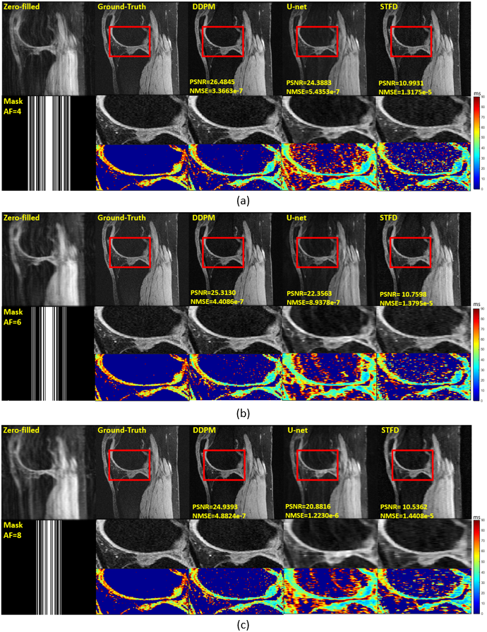
Fig2 shows representative reconstructed T1ρ-weighted images and T1ρ map in sagittal views. We compared three methods, a compressed sensing method(STFD⁹), CNN with U-net¹⁰, and DDPM. For U-net model, only one random sampling pattern was used for training. Given the high resolution, the SNR is relatively low. Both STFD and U-net artificially enlarge the cartilage region and underestimate the T1rho values. The DDPM is superior based on PSNRS and NMSE and the quantitative maps are very close to the ground truth. U-net performance can be similar to DDPM if training is repeated for each sampling pattern for each echo and reduction factor. In contrast, DDPM only needs to be trained once and then used for all sampling patterns.

Conclusion

In this abstract, we studied the use of DDPM for accelerated T1ρ imaging. T1ρ parameter maps from the DDPM show improvement over the competing methods while the training only needs to be performed once. More data sets will be used for evaluating tissue quantification accuracy in future studies.

References

[1] Ying L, Liang ZP. Parallel MRI using phased array coils (2010) IEEE Signal Processing Magazine, 27 (4), pp. 90-98.
[2] Zhou Y, Pandit P, Pedoia V, Rivoire J, Wang Y, Liang D, Li X, Ying L. (2016), Accelerating t1ρ cartilage imaging using compressed sensing with iterative locally adapted support detection and JSENSE. Magn. Reson. Med, 75: 1617-1629. https://doi.org/10.1002/mrm.25773
[3] Li H, Yang M, Kim J, Liu R, ZhangC, Huang P, Gaire S, Liang D, Li X, Ying L. Ultra-fast Simultaneous T1rho and T2 Mapping using Deep Learning, International Society of Magnetic Resonance in Medicine Annual Meeting, #2669, Aug 2020.
[4] Wang S, et al. Accelerating magnetic resonance imaging via deep learning, 2016 IEEE 13th International Symposium on Biomedical Imaging (ISBI), 2016, pp. 514-517, doi: 10.1109/ISBI.2016.7493320.
[5] Chung H, et al. Score-based diffusion models for accelerated MRI. arXiv: 2110.05243,2022.
[6] Cao C, Cui Z, Liu S, Liang D, Zhu Y. (2022). High-Frequency Space Diffusion Models for Accelerated MRI. arXiv. https://doi.org/10.48550/arXiv.2208.05481
[7] Xie Y and Li Q. Measurement-conditioned denoising diffusion probabilistic model for under-sampled medical image reconstruction. arXiv preprint arXiv:2203.03623, 2022.
[8] Liu R, Kim JH, Li H, Huang P, Li X, Ying L. Highly Accelerated Multi-channel 3D Knee Imaging Using Denoising Diffusion Probabilistic Model (DDPM) and GRAPPA, International Society of Magnetic Resonance in Medicine Annual Meeting, #4044, May 2023.
[9] Zibetti MVW, Sharafi A, Otazo R, Regatte RR. Accelerating 3D-T1ρ mapping of cartilage using compressed sensing with different sparse and low-rank models. Magn Reson Med. 2018 Oct;80(4):1475-1491. doi: 10.1002/mrm.27138. Epub 2018 Feb 25. PMID: 29479738; PMCID: PMC6097944.
[10] Li H, Yang M, Kim JH, et al. SuperMAP: Deep ultrafast MR relaxometry with joint spatiotemporal undersampling. Magn Reson Med. 2023; 89: 64-76. doi:10.1002/mrm.29411