Introduction

Cine cardiac MRI is used to evaluate cardiac functions and vascular abnormalities [1]. However, MRI requires a long scan time, which inevitably induces motion artifacts [7]. Recently, diffusion-based generative methods [2-4] have shown promising results. In this work, we trained a diffusion-based model with simulated data from ACDC dataset [5] to reduce the cine cardiac MRI motion artifacts. We then compared the results using the proposed method with results using state-of-the-art methods.

Method

Diffusion Model
Given a data distribution $$$x_0\sim q\left(x_0\right)$$$, the forward process in which we add Gaussian noise to in T steps, producing a sequence of noisy samples $$$x_1,\ldots,x_T$$$. Then, we can factorize the joint distribution of $$$x_1,x_2,\ldots,x_T$$$ conditioned on $$$x_0$$$ into:
$$q\left(x_t\middle| x_{t-1}\right)=\mathcal{N}\left(x_t;\sqrt{1-\beta_t}x_{t-1},\beta_tI\right)$$
The reverse diffusion is parameterized by a prior distribution $$$p\left(x_T\right)=\mathcal{N}\left(x_T;0,I\right)$$$ and a parameter $$$p_\theta\left(x_{t-1}|x_t\right)$$$. We choose the prior distribution $$$p\left(x_T\right)=\mathcal{N}\left(x_T;0,I\right)$$$. The parameter $$$p_\theta\left(x_{t-1}|x_t\right)$$$ takes the form of:
$$p_\theta\left(x_{t-1}\middle|x_t\right)=\mathcal{N}\left(x_{t1};\mu_\theta\left(x_t,t\right),\Sigma_\theta\left(x_t,t\right)\right)$$
where $$$\theta$$$ denotes model parameters, and the mean $$$\mu_\theta\left(x_t,t\right)$$$ and variance $$$\Sigma_\theta\left(x_t,t\right)$$$ are parameterized by neural networks. With the reverse process, we can generate a data sample $$$x_0$$$ by first sampling a noise vector $$$x_T \sim p\left(x_T\right)$$$, then iteratively sampling from the learnable parameter $$$x_{t-1} \sim p_\theta\left(x_{t-1}\middle| x_t\right)$$$ until $$$t\ =\ 1$$$. Each refinement step during inference is:
$$x_{t-1}=\frac{1}{\sqrt{\alpha_t}}\left[x_t-\frac{\beta_t}{\sqrt{1-\overline{\alpha}_t}}\epsilon_{\hat{\theta}}\left(x_t,t\right)\right]+\sigma_t z$$
In our study, we have access to both motion-corrupted image $$$y$$$ and motion-free image $$$x_0$$$. We optimize a neural denoising model $$$f_\theta$$$ that takes as input motion-corrupted image $$$y$$$ and a noisy image $$$x_T$$$, and aims to recover the noiseless image $$$x_0$$$. We define the inference process in terms of Gaussian conditional distributions, $$$p_\theta\left(x_{t-1}\middle| x_t,y\right)$$$. If the noise variance of the forward process steps is as small as possible, the optimal reverse process will be approximately Gaussian. Thus, each refinement step takes the form:
$$x_{t-1}=\frac{1}{\sqrt{\alpha_t}}\left[x_t-\frac{\beta_t}{\sqrt{{\overline{\alpha}}_t}}f_\theta\left(x_t,t,y\right)\right]+\sigma_tz$$

ACDC Synthetic Dataset
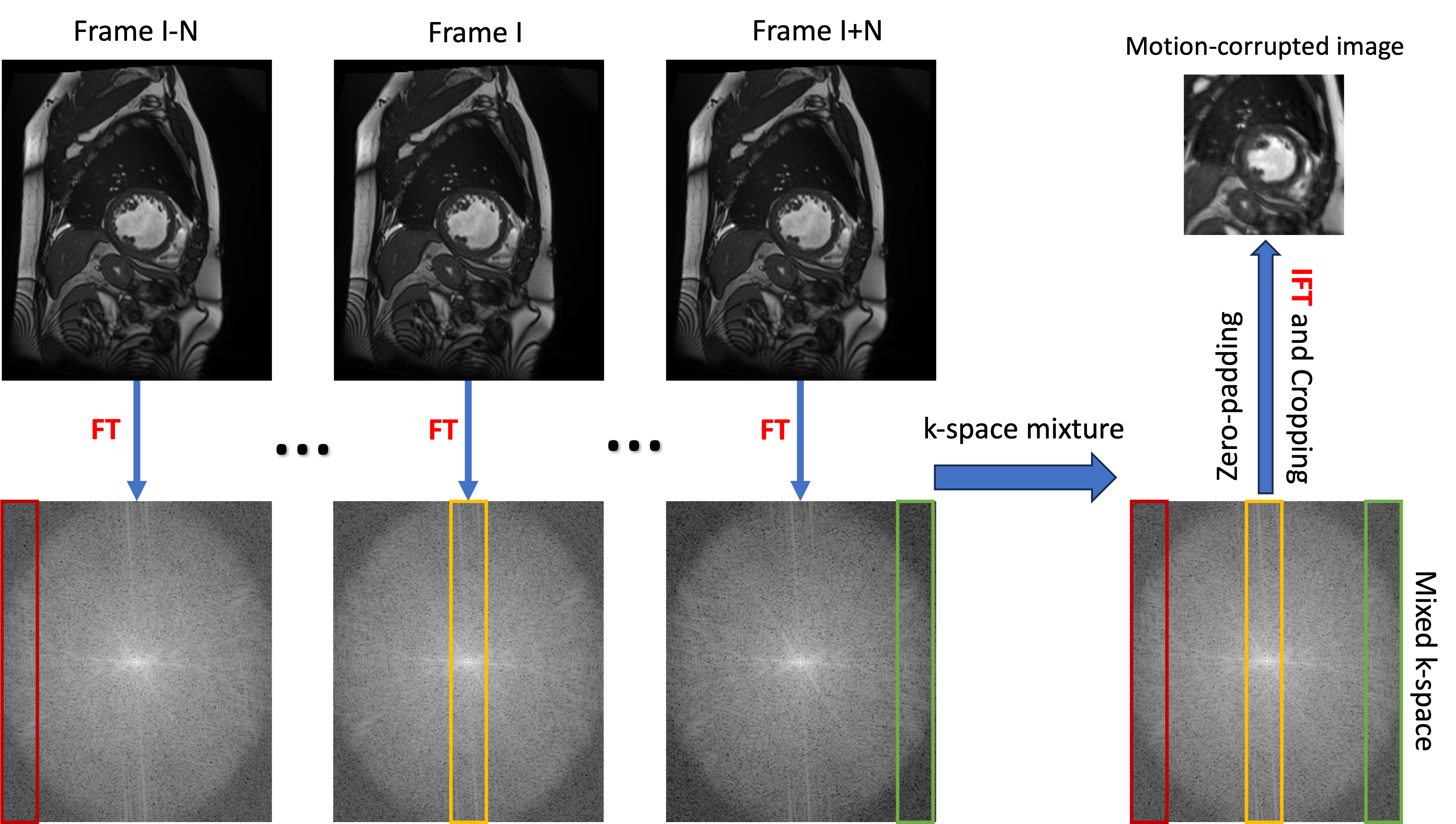
To create a dataset with paired motion-corrupted and motion-free data, we used all origin images from the ACDC dataset [5]. Based on these data, we synthesized motion-corrupted data by a simulation process similar to the approach outlined in [6]. Fig.1 provides an illustration of the process of synthesizing motion-corrupted images. We initially transformed each image into k-space using a Fourier transform. We then selected a set of 2N+1 consecutive frames and extracted an equal number of frequency encoding line data from each k-space and combined this line data to create a new k-space. Subsequently, we applied under-sampling and zero-padding to each new k-space, retaining only 25% of the data. Finally, we obtained the motion-corrupted images by performing an inverse Fourier transform.

Volunteer Study
To assess the model's performance with actual cardiac cine images, we conducted a volunteer study. The MR data was acquired using a 3T MR scanner (uMR 890, United Imaging, Shanghai, China). We examined five healthy subjects, obtained paired sets of motion-free and motion-corrupted images using a 2D SSFP sequence. These images were captured during breath-holding and encompassed five slice locations, including three short-axis views and two long-axis views. Additional imaging parameters included a FOV measuring 225mm × 300mm, a slice thickness of 8mm, TR/TE of 3ms/1.3ms.

Implementation Details
In this study, the method was trained on a dataset consisting of 14,100 images. For generating motion-corrupted images, we set N=7, using the motion-free images from the ACDC dataset. During the network training, the batch size was set to 24, and the network input dimensions were configured as 128 × 128. The training process involved 2,000 steps, and the DDIM model was utilized to expedite the sampling steps during inference, with a specified number of 100 steps.

Result and Discussion

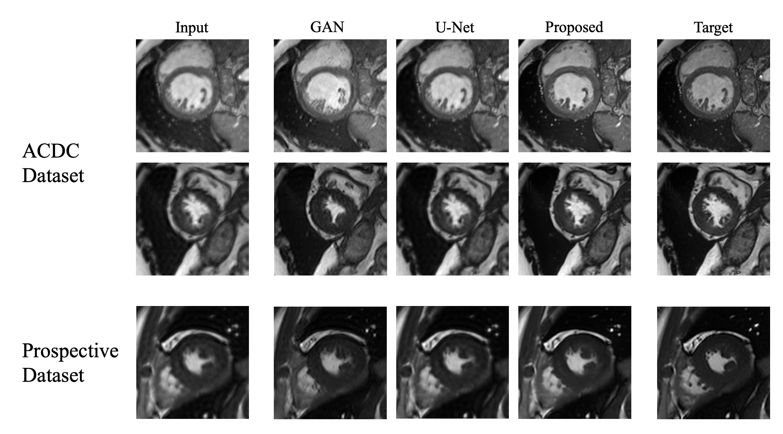
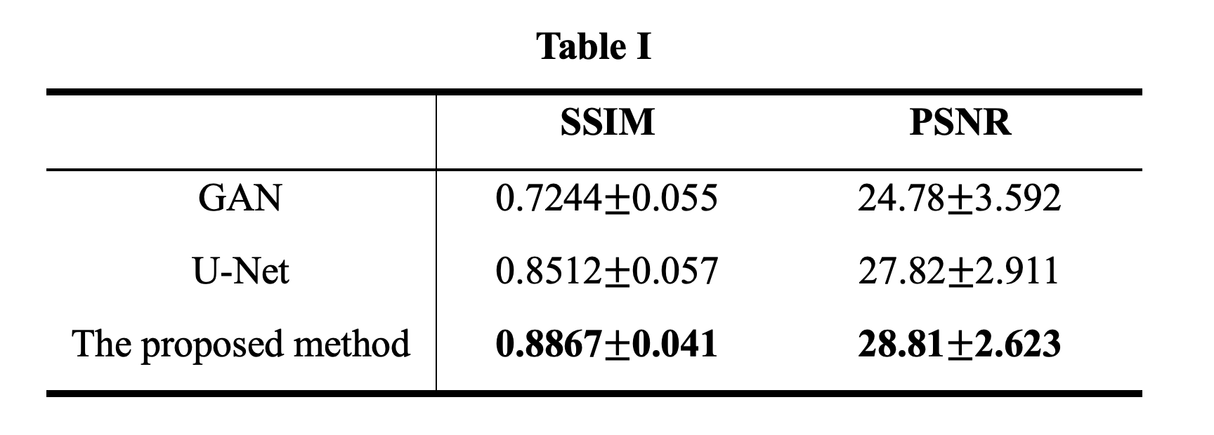
We conducted a comparative analysis of our proposed approach with two other methods: GAN and U-Net. As illustrated in Fig.2 and Table I, the results across both the ACDC synthetic dataset and the prospective dataset clearly indicates that the GAN and U-Net methods yield relatively inferior outcomes. In contrast, our method excels in producing results that closely approach the ground-truth, achieving the highest SSIM score of 0.8867 and PSNR score of 28.81 among all the evaluated methods. By calculation, we find that the p-value of proposed method with U-Net on PSNR is 3.1e-08, and on SSIM is 1.2e-21, and with GAN on PSNR is 5.2e-08, and on SSIM is 3.6e-206.

Conclusion

Our proposed method has shown significant improvements compared to existing methods. Through our approach, Fig.2, and Table I, we can achieve higher SSIM and PSNR values, indicating the effectiveness of our proposed method in preserving image quality. The results obtained from our experiments on the ACDC and prospective datasets consistently demonstrated the effectiveness and robustness of our proposed network.

References

1. Kellman, Peter et al. “High spatial and temporal resolution cardiac cine MRI from retrospective reconstruction of data acquired in real time using motion correction and resorting.” Magnetic resonance in medicine vol. 62,6 (2009): 1557-64. doi:10.1002/mrm.22153
2. Ho, Jonathan, Ajay Jain, and Pieter Abbeel. "Denoising diffusion probabilistic models." Advances in neural information processing systems 33 (2020): 6840-6851.
3. Song, Yang, and Stefano Ermon. "Generative modeling by estimating gradients of the data distribution." Advances in neural information processing systems 32 (2019).
4. Song, Yang, et al. "Score-based generative modeling through stochastic differential equations." arXiv preprint arXiv:2011.13456 (2020).
5. Bernard, Olivier, et al. "Deep learning techniques for automatic MRI cardiac multi-structures segmentation and diagnosis: is the problem solved?" IEEE transactions on medical imaging 37.11 (2018): 2514-2525.
6. Lyu Q, Shan H, Xie Y, et al. Cine Cardiac MRI Motion Artifact Reduction Using a Recurrent Neural Network. IEEE Trans Med Imaging. 2021;40(8):2170-2181. doi:10.1109/TMI.2021.3073381
7. Zaitsev, Maxim, Julian Maclaren, and Michael Herbst. "Motion artifacts in MRI: A complex problem with many partial solutions." Journal of Magnetic Resonance Imaging 42.4 (2015): 887-901.