Introduction

Deep neural networks^1,2,3 (DNNs) have demonstrated remarkable efficiency in reconstructing undersampled k-space data. Furthermore, models incorporating physics-guided self-supervised DNNs^4,5 have reliably reconstructed images utilizing limited data. However, the integration of radial k-space data⁶ into these methodologies has not been explored enough. Being more robust to motion artifacts and allowing for a more uniform k-space sampling along time⁷, radial k-space data offers a considerable advantage over Cartesian data for MR scans of moving organs, such as the heart.

In this work, we propose a physics-guided self-supervised DNN model designed to reconstruct radially sampled cardiac MR images using a novel regularizer. The contributions of this work are twofold: Firstly, the proposed model pioneers self-supervision for radial MR acquisitions, harnessing the advantages of radial data and allowing for efficient learning on very limited amounts of acquisitions. Secondly, our approach enhances the DNN architecture for improved cardiac motion capture by integrating a low-rank and sparse denoiser, significantly improving MR reconstruction for moving organs.

Methods

Cardiac MRI measurements are obtained alongside the patient’s electrocardiogram signal, which may span multiple cardiac cycles. 8 slices were acquired from 16 volunteer subjects, totaling 128 samples, on a 1.5T Philips machine using a 28-channel cardiac coil, consisting of short axis heart scans. The acquisition was conducted on 8 mm slice thickness, 2x2 mm$$$^2$$$ resolution, TE/TR = 1.16/2.3 ms, b-SSFP, radial tiny golden angle, 20s nominal scan time and breath-hold acquisition. The measurements are aligned into a unified cardiac cycle in order to mitigate the sparsity of the radial acquisitions in the spatial-frequency dimensions. They are then organized into temporal windows, each of which corresponds to a distinct cardiac phase of the heartbeat. Two datasets were considered in this work, using one and four cardiac cycles.

Our proposed model builds upon the self-supervised physics-guided MR reconstruction framework⁵, to solve the non-linear inverse problem by variable-splitting via quadratic penalty through iterative data consistency (DC) and regularizer (denoiser) steps:

$$l^{(i)}, s^{(i)} = f(y_\Omega, E_\Omega; \phi),\\
x^{(i)} = x^{(i-1)} - \mu E^{H}_{\Omega}(E_{\Omega}(l^{(i)}+s^{(i)})-y_\Omega).$$

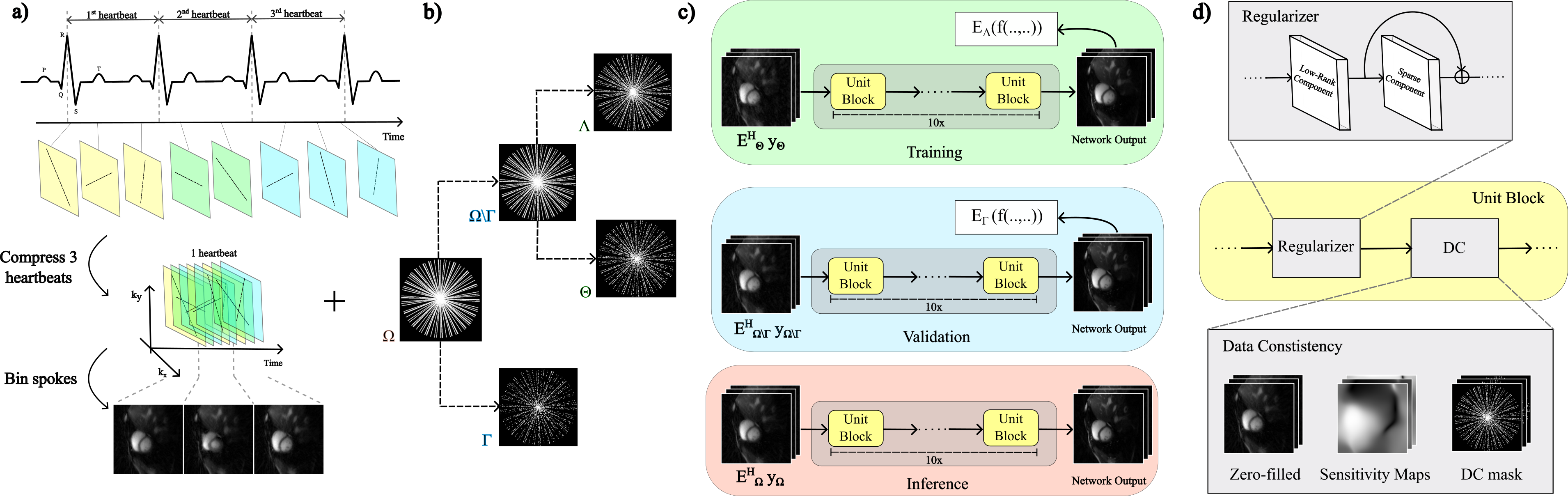
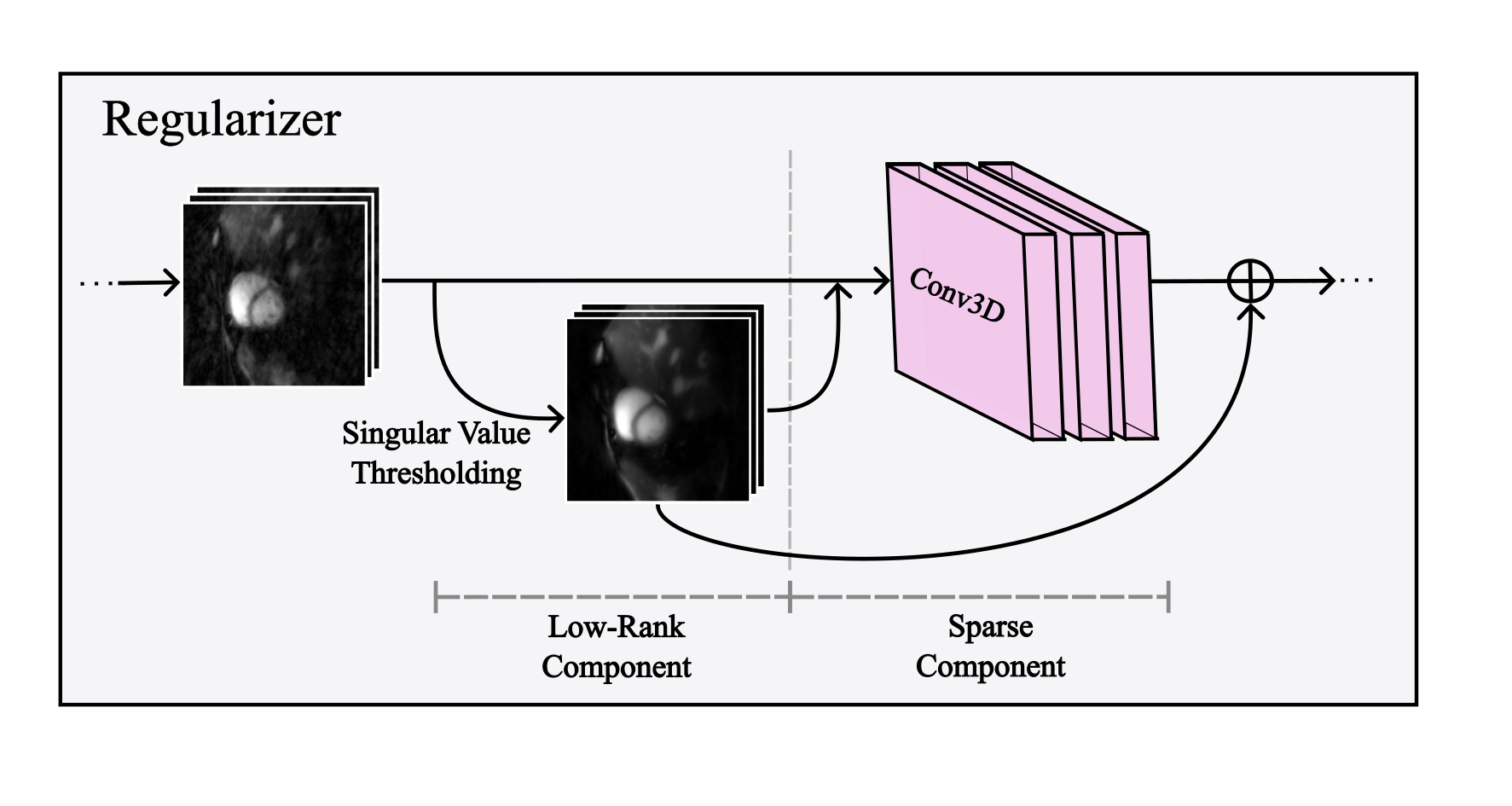
Function $$$f$$$ represents the regularizer parameterized by $$$\phi$$$. To further leverage the intrinsic low-rank property of dynamic images, the regularizer incorporates a learnable low-rank and sparse component, $$$l^{(i)}$$$ and $$$s^{(i)}$$$, for an iteration $$$(i)$$$. $$$y_\Omega$$$ is the input k-space, masked by the undersampling mask $$$\Omega$$$, and the corresponding forward operator $$$E_\Omega$$$. Thus, the denoiser captures moving (heart motion) and non-moving parts (e.g. ribs, liver) of the image more efficiently than through a regular convolutional neural network⁵ (CNN). Figure 2 shows an in-depth illustration of the regularizer. The second equation represents the DC step, which uses a conjugate gradient approach. $$$\mu$$$ is a regularizing parameter, $$$H$$$ represents the Hermitian and $$$x$$$ is the reconstructed image. The regularizer-DC pairs are depicted in Figure 1d inside the unit block.

The proposed architecture supports supervised and self-supervised tasks. The model receives its self-supervision signal by subsampling the initial undersampling mask $$$\Omega$$$ (Figure 1a). During validation, $$$\Omega$$$ is split into two distinct subsets: $$$\Gamma$$$ for the loss calculation and $$$\Omega\setminus\Gamma$$$ for the model input. Subsampled from $$$\Omega\setminus\Gamma$$$, masks $$$\Theta$$$ and $$$\Lambda$$$ follow the same pattern during training time, resulting in the following loss:

$$ \operatorname*{min}_\phi \frac{1}{N} \sum_{n=1}^N L(y_{\Lambda}^n, E_{\Lambda}^n (f(y_\Theta^n, E_\Theta^n; \phi)))$$

Figure 1b,c shows a full overview of the self-supervised masking and training strategy. The proposed model is evaluated in both supervised and self-supervised tasks and compared to an iterative regularized reconstruction method (CG Sense⁸), a compressed sensing method (L+S⁹), and to the supervised and self-supervised models described in Yaman et al.⁵, adapted to radial k-space. The predictions are compared on normalized mean squared error, structural similarity index and peak signal-to-noise-ratio to the 20 heartbeat iterative L+S reconstruction.

Results

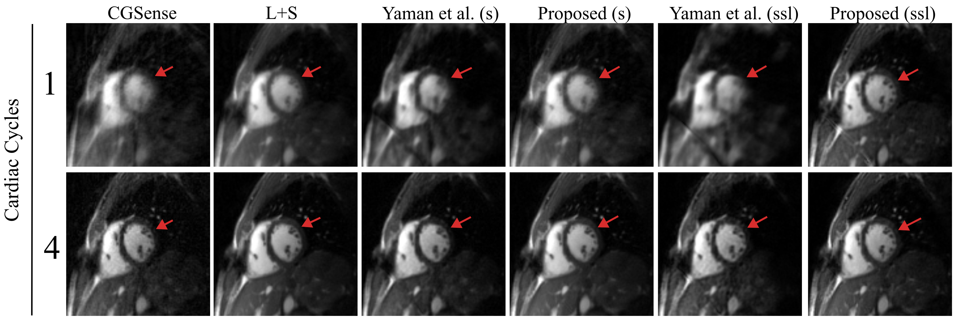
The proposed method outperforms the other reconstruction techniques in all metrics for one and four cardiac cycle datasets (Table 1). Figure 3 shows that our method surpasses the others in keeping the noise and streaking artifacts low. Moreover, higher contrast is achieved by the methods exploiting the low-rank prior of dynamic images across both datasets (red arrow). The temporal profiles and their errors are shown in Figure 4, where the proposed method achieves the lowest error and a smoother reconstruction on the temporal dimension.

Discussion and Conclusion

This work introduces a physics-guided self-supervised model architecture to efficiently train on small amounts of dynamic radially sampled data. Adding learnable low-rank and sparse components to the architecture dramatically improves the performance of the models for cardiac reconstruction, while CNNs as regularizers deliver sub-par performance. We anticipate that further development in the area of data preparation for patients with arrhythmia will expand its potential applications.

Acknowledgements

No acknowledgement found.