4477
Simultaneous Measurement of CEST and $$$T_1$$$ using Model-based Multi-Pool-Lorentzian Look-Locker Reconstruction1Institute of Biomedical Imaging, Graz University of Technology, Graz, Austria, 2Institute of Neuroradiology, Friedrich-Alexander-Universität Erlangen-Nürnberg (FAU), University Hospital Erlangen, Erlangen, Germany, 3High-Field Magnetic Resonance Center, Max-Planck Institute for Biological Cybernetics, Tübingen, Germany
Synopsis
Keywords: CEST / APT / NOE, CEST & MT, Lorentzian, Model-based Reconstruction
Motivation: Conventional quantitative CEST experiments require the additional determination of $$$T_1$$$. CEST sequences include $$$T_1$$$ relaxation periods that can be exploited to estimate $$$T_1$$$ simultaneously to the CEST parameters.
Goal(s): The development of a technique for efficient simultaneous quantification of CEST contrast and $$$T_1$$$.
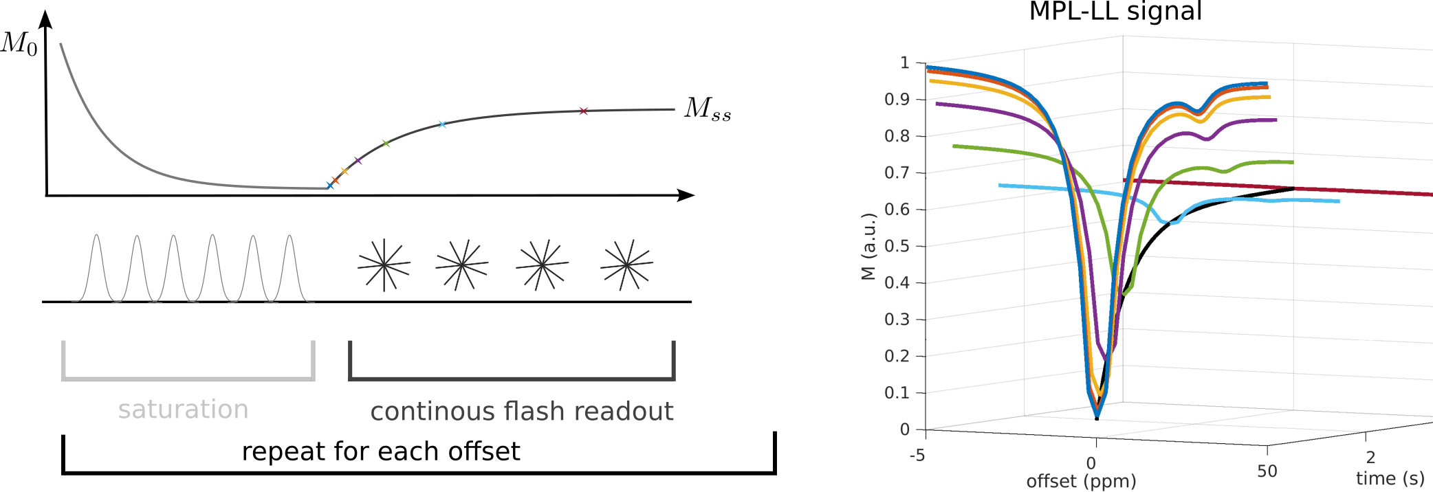
Approach: Integration of a FLASH acquisition train after conventional CEST saturations. Simultaneous CEST contrast and $$$T_1$$$ fitting is achieved by extending the Lorentzian model of the CEST spectrum with a Look-Locker model for the FLASH readout.
Results: The proof-of-concept was implemented, and first results are demonstrated in a two pools phantom and a four pool in vivo study.
Impact: The presented technique enables calculating $$$T_1$$$ corrected quantitative CEST results from one measurement. This simplifies the application of the apparent exchange-dependent relaxation ($$$MTR_{AREX}$$$), the quasi-steady-state$$$\;$$$contrast and other CEST metrics, which require a $$$T_1$$$ map, making them more accessible.
Introduction
Chemical Exchange Saturation Transfer (CEST) offers insights into the metabolism and numerous pathologies. A generic quantification can be performed with Multi-Pool Lorentzian (MPL) fitting, which exploits Lorentzian-lineshapes to describe the Z-spectrum1. The resulting contrasts strongly depend on the underlying $$$T_1$$$ relaxation and saturation of the tissue. They can be compensated with the apparent exchange-dependent relaxation ($$$MTR_{AREX}$$$)2 or the quasi-steady-state contrast (QUASS)3, respectively. Both corrections require an accurate $$$T_1$$$ map that is conventionally calculated from additional measurements2,3 that prolong these acquisitions and can introduce additional errors such as motion. In this work, we propose a technique for the simultaneous measurement of CEST and $$$T_1$$$ by adding continuous FLASH$$$\;$$$readouts to conventional CEST sequences encoding the required $$$T_1$$$ information and avoiding additional scans. We extend MPL with a Look-Locker (LL) model4 to make use of the $$$T_1$$$ sensitivity of the sequence.$$$\;$$$We demonstrate the application of the developed technique in a phantom and in vivo study calculating $$$MTR_{AREX}$$$ and QUASS$$$\;$$$rom the resulting CEST parameters$$$\;$$$and$$$\;$$$$$$T_1$$$ maps.Theory
In CEST measurements the magnetization after saturation can be described$$$\;$$$as$$M(\omega)=M_0 \left(1-\sum_{i=0}^{N-1}L_i(\omega)\right)$$with $$$N$$$ Lorentzian lineshapes$$L_i(\omega)=a_i \frac{{(\Gamma_i/2)}^2}{{(\Gamma_i/2)}^2+(\omega-\omega_{0i})}$$defined with their equilibrium magnetization $$$M_0$$$, offset frequency $$$\omega$$$, amplitude $$$a_i$$$, width $$$\Gamma_i$$$, and frequency shift $$$\omega_{0i}$$$1.In the proposed Multi-Pool$$$\;$$$Lorentzian$$$\;$$$Look-Locker (MPL-LL) technique$$$\;$$$a$$$\;$$$FLASH$$$\;$$$based$$$\;$$$readout$$$\;$$$scheme is incorporated after saturation of the magnetization.The signal acquired during this excitation train is proportional to $$$M_z$$$ and can be modeled with a Look-Locker signal model4:$$M(t)=M^*-(M^* - M(\omega))\exp{\left(-\frac{t}{T^*_1}\right)}.$$Here,$$$\;$$$$$$M^*$$$ is the steady-state magnetization, $$$T_1^*$$$$$$\;$$$is the effective longitudinal relaxation time constant and $$$t$$$$$$\;$$$denotes the time after saturation.$$$\;$$$By introducing the$$$\;$$$steady-state$$$\;$$$fraction $$$f_{ss}=\frac{M^*}{M_0}$$$the combined MPL-LL signal$$$\;$$$model can be described with$$M(t,\omega) = M_0\left( f_{ss}-\left( f_{ss}-1+\sum_{i=0}^{N-1}L_i(\omega)\right)\exp{\left(-\frac{t}{T^*_1}\right)} \right).$$ $$$T_1$$$$$$\;$$$is estimated from $$$T_1^*$$$ and $$$f_{ss}$$$ following$$T_1 = \frac{T_1^*}{f_{ss}} .$$The MPL-LL signal model is incorporated in the following non-linear problem and solved for parameter identification:$$\hat{u}=argmin_u||\mathcal{P}\mathcal{F}\mathcal{C}M(t,\omega,u)-d_k||^2_2+\gamma TGV_j(u)$$with the measured$$$\;$$$k-space$$$\;$$$data $$$d_{k}$$$, the parameter$$$\;$$$vector $$$u=M_0~f_{ss}~T_1^*~a_i\Gamma_i~\omega_i)^T$$$, the weighting$$$\;$$$parameter $$$\gamma$$$ for the joint total generalized variation $$$TGV_j(u)$$$ regularization5,6, the$$$\;$$$coil operator $$$\mathcal{C}$$$, the$$$\;$$$Fourier operator $$$\mathcal{F}$$$ and the pattern operator $$$\mathcal{P}$$$.
Methods
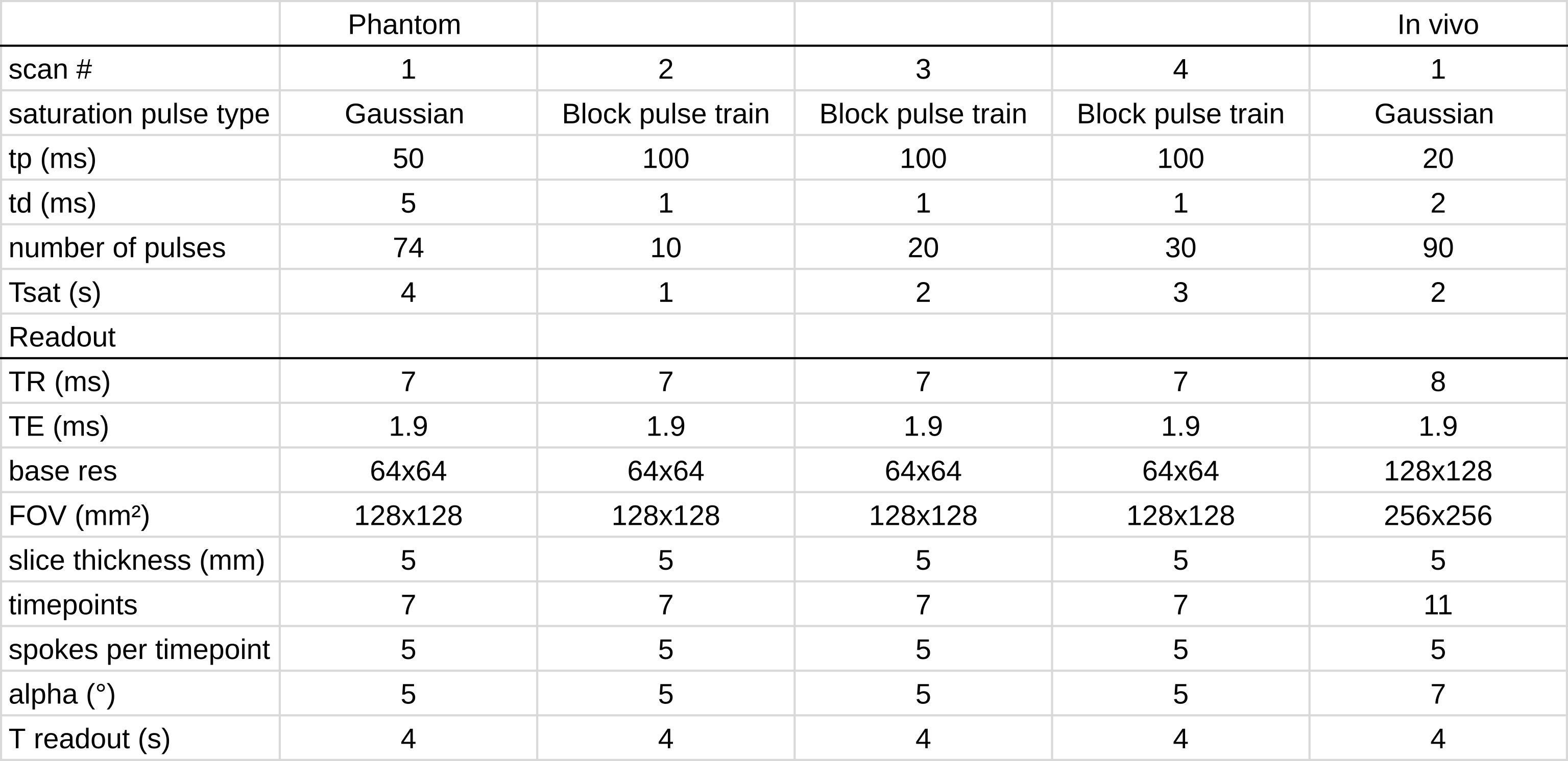
A phantom consisting of$$$\;$$$nine$$$\;$$$falcon tubes was constructed. Water with Nicotinamid (NA) in three different concentrations (100, 150 and 200 mM) were doped with Gadovist (Bayer Vital GmbH, Leverkusen, Germany) to create a range of $$$T_1$$$.The MPL-LL sequence was implemented using the pulseq-CEST toolbox7 in MATLAB (2022b, Mathworks, Natick, MA). All measurements were acquired on a MAGNETOM$$$\;$$$Vida$$$\;$$$3T scanner (Siemens$$$\;$$$Healthcare$$$\;$$$GmbH,$$$\;$$$Erlangen,$$$\;$$$Germany) using a 20 channel head-coil. In total, four MPL-LL scans of the phantom and one Inversion-Recovery (IR) FLASH $$$T_1$$$ reference measurement8 were performed. An additional in vivo MPL-LL measurement with an IR FLASH $$$T_1$$$ reference scan and a reference CEST measurement were acquired. Sequence parameters for the MPL-LL scans can be found in Figure 2.
The model-based reconstruction was performed using the PyQMRI toolbox$$$\;$$$9. It exploits the Iteratively Regularized Gauss-Newton Method (IRGNM) combined with a primal-dual splitting algorithm to solve the non-linear problem$$$\;$$$10. The post-processing was implemented with MATLAB and calculated $$$T_1$$$, Lorentzian-based $$$MTR_{REX}$$$ and $$$MTR_{AREX}$$$ at 3.5ppm2, and the quasi-steady-state contrast (QUASS)3.
Results and Discussion
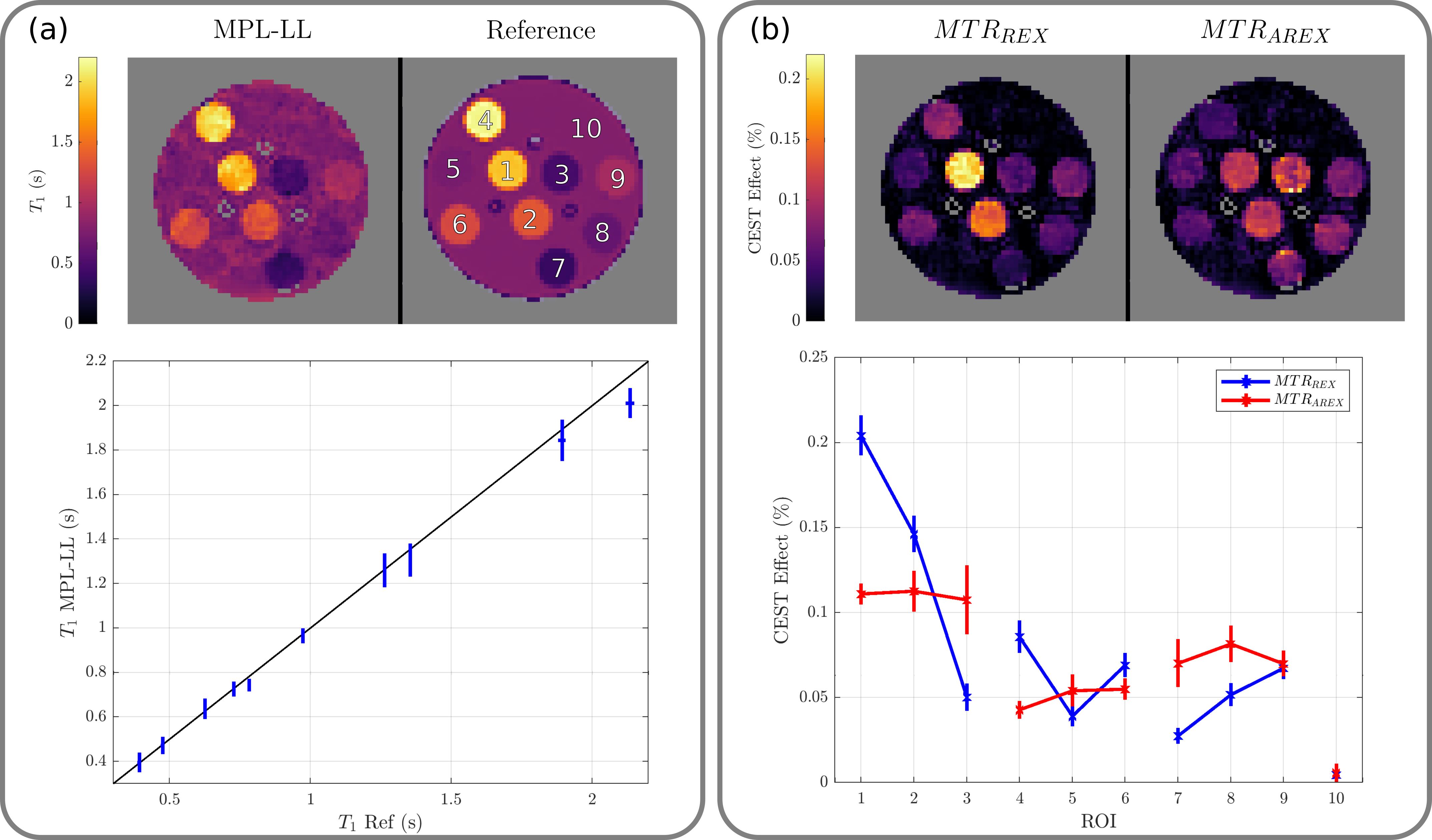
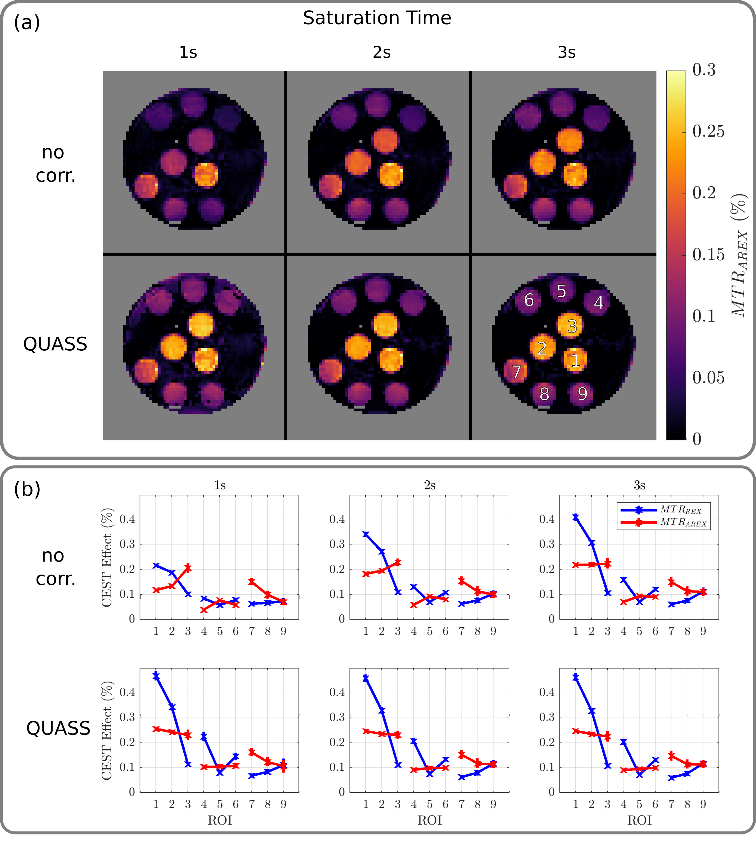
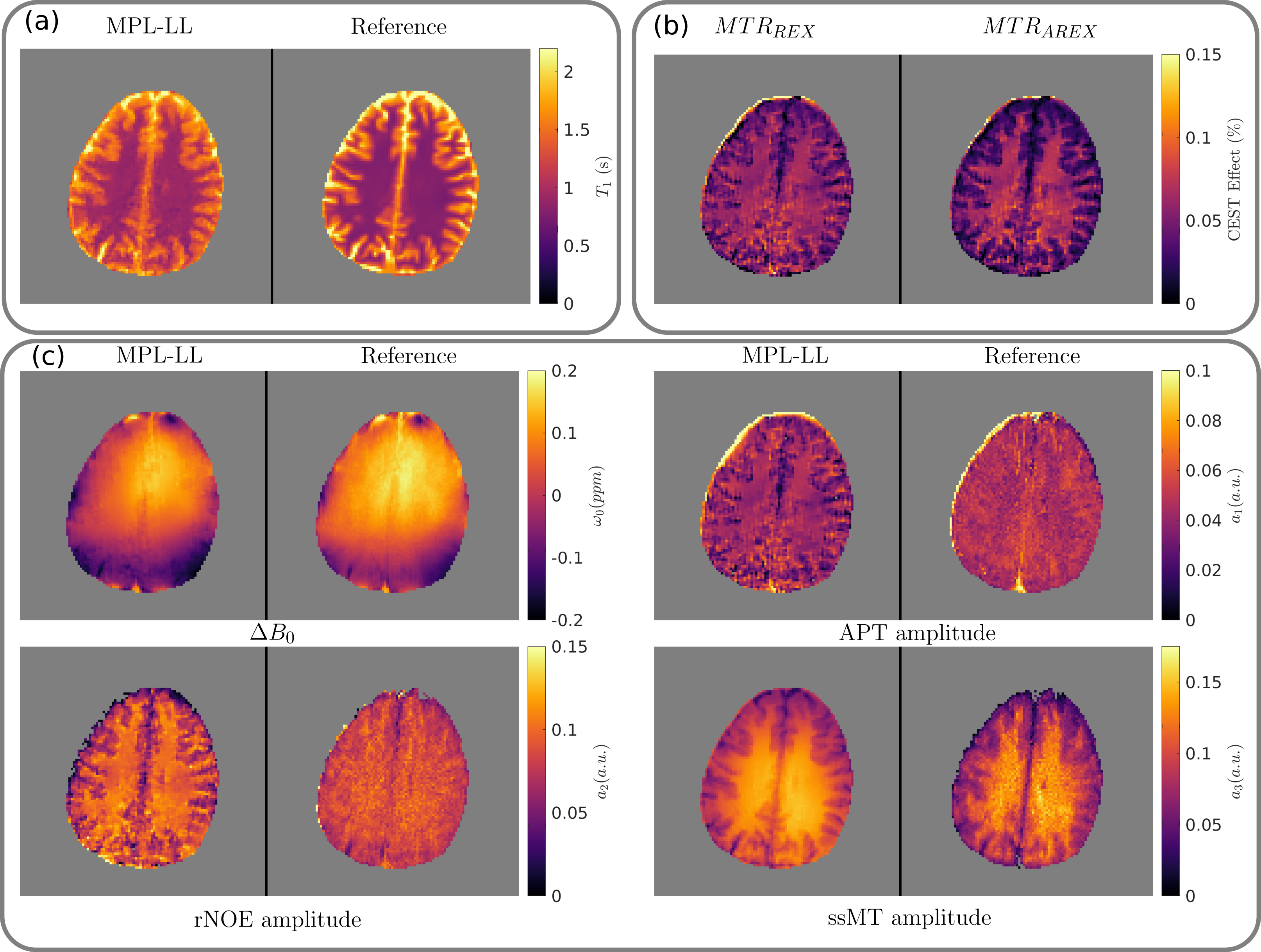
In$$$\;$$$Figure$$$\;$$$3$$$\;$$$the$$$\;$$$results$$$\;$$$for $$$T_1$$$, $$$MTR_{REX}$$$ and $$$MTR_{AREX}$$$ of the$$$\;$$$tube phantom$$$\;$$$measurements are depicted. Ten ROIs (tubes and background) were compared to the reference measurement and show good agreement for $$$T_1$$$ except for the highest values of over two seconds. $$$MTR_{REX}$$$$$$\;$$$shows the influence of$$$\;$$$$$$T_1$$$ on the CEST$$$\;$$$contrast, with four times higher values between ROI one and three for the same NA concentration. This is corrected in $$$MTR_{AREX}$$$ based on the fitted $$$T_1$$$.$$$\;$$$In Figure 4 the application of the QUASS correction is shown by using different saturation times for each measurement.$$$\;$$$Here,$$$\;$$$$$$MTR_{AREX}$$$ is not applicable, as the steady-state is not yet reached, which results in inconsistent values over the tubes with the same NA concentration. This influence is reduced by applying the QUASS correction based on the fitted $$$T_1$$$ map, which enables shorter overall measurement times.$$$\;$$$Figure 5 presents in$$$\;$$$vivo measurements using the MPL-LL sequence and reconstruction. The MPL-LL $$$T_1$$$ exhibits values close to the reference method. $$$MTR_{REX}$$$$$$\;$$$and $$$MTR_{AREX}$$$ are shown as well as selected parameter maps in comparison to a conventional CEST measurement. $$$\Delta$$$$$$B_0$$$ shows good agreement between the methods. For$$$\;$$$the$$$\;$$$fitted amplitudes the$$$\;$$$MPL-LL method results in sharper tissue boundaries, especially visible in$$$\;$$$ssMT. The time encoding of the acquisition mitigates the blurring artifact associated with the long single-shot acquisitions used in conventional CEST imaging.Conclusion
This work presented$$$\;$$$a$$$\;$$$convenient$$$\;$$$and$$$\;$$$time-efficient extension of conventional CEST$$$\;$$$ experiments with $$$T_1$$$ encoding FLASH readouts. The underlying signal model for the developed MPL-LL technique is derived and exploited to simultaneously quantify CEST contrast and $$$T_1$$$ maps. Initial results on phantom and in vivo experiments are presented with their calculated $$$MTR_{AREX}$$$ or QUASS contrasts, all corrected without the need of additional scans.Acknowledgements
No acknowledgement found.References
1. M Zaiss et al., Quantitative separation of CEST effect from magnetization transfer and spillover effects by Lorentzian-line-fit analysis of z-spectra. J Magn Reson, 211(2), 2011.
2. M Zaiss et al., Inverse Z-spectrum analysis for spillover-, MT-, and T1-corrected steady-state pulsed CEST-MRI – application to pH-weighted MRI of acute stroke. NMR in Biomedicine, 27(3), 2014.
3. PZ Sun, Quasi-steady-state chemical exchange saturation transfer (QUASS CEST) analysis—correction of the finite relaxation delay and saturation time for robust CEST measurement. Magn Reson Med, 85(6), 2021.
4. DC Look and DR Locker, Time Saving in Measurement of NMR and EPR Relaxation Times. Rev Sci Instr, 41(2), 1970.
5. O Maier et al., Robust Lorentzian fitting of CEST spectra utilizing joint spatial regularization. Proc 30 Annual Meeting ISMRM, 30, 2022.
6 K Bredies et al., Total generalized variation. SIAM J Imag Sci, 3(3), 2010.
7. K Herz et al., Pulseq‐CEST: Towards multi‐site multi‐vendor compatibility and reproducibility of CEST experiments using an open‐source sequence standard. Magn Reson Med, 86(4), 2021.
8. X Wang et al. Model-based T1 mapping with sparsity constraints using single-shot inversion-recovery radial FLASH. Magn Reson Med 79(2), 2018.
9. O Maier et al., PyQMRI: An accelerated Python based Quantitative MRI toolbox. J Open Source Software 5(56), 2020.
10. A Chambolle and T Pock, A first-order primal-dual algorithm for convex problems with applications to imaging. J Math Imag Vis 40(1), 2011.
Figures