4465
Comparison of fast quantitative magnetization transfer imaging methods on a 1.5 T MR-Linac1Medical Biophysics, University of Toronto, Toronto, ON, Canada, 2Physical Sciences, Sunnybrook Health Sciences Centre, Toronto, ON, Canada, 3Department of Radiation Oncology, Sunnybrook Health Sciences Centre, Toronto, ON, Canada, 4Medical Imaging, University of Toronto, Toronto, ON, Canada, 5Medical Imaging, Sunnybrook Health Sciences Centre, Toronto, ON, Canada
Synopsis
Keywords: Magnetization Transfer, Magnetization transfer, MR-Linac
Motivation: Quantitative magnetization transfer (qMT) could guide radiotherapy on MRI-linear accelerators (MR-Linacs), but limited scan time requires a fast sequence. Fast 3D qMT is possible with balanced steady-state free precession (bSSFP) or echo-planar imaging (EPI), but which method is superior is unclear.
Goal(s): Our goal was to determine whether bSSFP or EPI qMT on a 1.5T MR-Linac was best for imaging glioblastoma patients.
Approach: Eight patients were scanned using both methods. Repeatability in normal tissue and magnitude of tumor changes were compared.
Results: A 2 minute 20 second EPI qMT scan was more repeatable than bSSFP qMT and detected greater tumor changes.
Impact: The improvement in quantitative magnetization transfer acquisition speed through using 3D EPI enables integration into MR-Linac radiotherapy workflows, an unmet need as qMT can detect white matter changes which could be used to assess tumor response during treatment.
Background
MR-linear accelerators (MR-Linacs) enable daily imaging for radiotherapy adaptation1, which could improve outcomes for glioblastoma patients through radiation dose escalation to radioresistant regions of tumor or through reducing treatment margins to minimize treatment-related toxicity. Quantitative magnetization transfer (qMT) imaging can detect early changes in white matter microstructures which could be used to assess tumor response2,3 and therefore guide adaptation. Volumetric qMT scans require long scan times due to needing multiple magnetization transfer (MT)-weighted images. We previously implemented a 3D balanced steady-state free precession (bSSFP) qMT scan on an MR-Linac4, though the quality of parameter maps was limited by MR-Linac hardware. In this abstract, we implement an alternative MR-Linac qMT sequence using 3D echo planar imaging (EPI) readouts and compare its repeatability and accuracy to the bSSFP-based sequence.Methods
Data acquisition: Eight glioblastoma patients received fractionated radiotherapy on a 1.5T MR-Linac (Unity, Elekta, Stockholm, Sweden). Whole-brain bSSFP-qMT and EPI-qMT images were acquired at weekly intervals and on separate days during treatment (Figure 1). 3D bSSFP-qMT scans had varying flip angle and RF pulse duration5 (flip angles=5-35°, TRF=0.672-6.669ms; 2×2×2mm3 resolution, scan time=8min). 3D EPI-qMT scans consisted of interleaved saturation-readout blocks (30ms Gaussian pulses, 39ms EPI readout, 1.5×1.5×8mm3 resolution, EPI factor=31, offset frequencies=250Hz-100kHz, MT pulse angles=1200°,1800°, scan time=2.33min). T1/B0/B1 maps necessary for fitting were acquired. T1-weighted scans were acquired for anatomical reference (3D MPRAGE, TR/TE=8.0/3.6ms, voxel size=1.1×1.1×2.2mm3).Fitting: The macromolecular fraction (F), free pool T2 (T2f) and exchange rate (kf), were estimated voxelwise using a nonlinear least-squares solver (MATLAB 2018b lsqcurvefit). bSSFP scans were fitted to the bSSFP qMT signal equation previously described5,6. EPI scans were fitted to a modified solution of the two-pool model under continuous wave irradiation7,8; the continuous wave power was set to the time-averaged MT power over the entire sequence. The free pool T1 was set using the T1 map. For bSSFP-qMT fits, the constraint kf=4.5 s-1 (kf in white matter5) was applied to stabilize the parameter fitting. For EPI-qMT fits, the signal was normalized to the signal at the greatest offset frequency to accelerate fitting.
Image processing: Four regions of interest were used: contralateral normal-appearing white and gray matter (cNAWM, cNAGM), cerebrospinal fluid (CSF), and the gross tumor volume (GTV). The cNAWM, cNAGM and CSF were automatically segmented from the T1-weighted scans with FSL FAST9 and restricted to the side of the brain contralateral to the tumor. The GTV was contoured at treatment planning using gadolinium enhanced T1-weighted images.
Data analysis: The median fitted parameter values within each ROI were calculated. Between-session repeatability in normal appearing brain regions (cNAWM, cNAGM) was calculated as previously described10, using a one-way random effects model to compute within-subject standard deviations (wSD) and coefficients of variation (wCV). bSSFP qMT and EPI qMT parameter maps that were acquired on consecutive treatment fractions (n=12) were compared. The relative change in macromolecular fraction within the GTV throughout treatment was also computed.
Results
An example of the fitted signal curves for both bSSFP and EPI qMT are shown in Figure 2. Exemplary ROIs and parameter maps are shown in Figure 3. Median parameter values have the expected white-matter/gray-matter contrast, though absolute values do not match literature11-13 (Figure 4A). EPI-qMT has a lower wCV across all parameters compared to bSSFP-qMT (Figure 4B). Macromolecular fraction values between the methods appear to be correlated in normal-appearing tissue (Figure 4C). Relative changes in macromolecular fraction within the GTV during treatment are greater in EPI-qMT compared to bSSFP-qMT (Figure 5).Discussion
Both bSSFP and EPI qMT have limited parameter accuracy. The accuracy of bSSFP-qMT may be affected by the exchange rate fitting constraint, the limited range of MT-weighted images and B0-banding artifacts (Figure 3B) which resulted from long TRs due to MR-Linac gradient limitations. The accuracy of EPI-qMT may be affected by the model used to fit the data. While the analytical solution appears to fit the data well, it may not accurately reflect the true magnetization of the system as it does not account for any steady-state magnetization. Fitting directly to the Bloch-McConnell simulations may yield more accurate parameter maps14. Additional T2 mapping for both methods may also support fitting.Compared to bSSFP-qMT, the EPI-qMT parameters in normal-appearing tissue had lower between-session variability. EPI-qMT may be more sensitive to changes during treatment as macromolecular fraction changes within the GTV during treatment were larger.
Conclusion
Fast, whole brain qMT was implemented on a 1.5T MR-Linac using 3D bSSFP and EPI sequences. The 2.33-minute EPI-qMT had fewer image artifacts, lower between-session variability, and was more sensitive to changes within the GTV.Acknowledgements
We thank the MR-Linac radiation therapists Shawn Binda, Danny Yu, Renée Christiani, Katie Wong, Helen Su, Monica Foster, Rebekah Shin, Khang Vo, Ruby Bola, Susana Sabaratram, Christina Silverson, Danielle Letterio, and Anne Carty for scanning and for their assistance with the protocol; Mikki Campbell for study coordination; and Brian Keller and Brige Chugh for MR-Linac operations. We gratefully acknowledge the following sources of funding: Natural Sciences and Engineering Research Council (NSERC), Canadian Institutes of Health Research (CIHR), Ontario ERA.References
[1] Y. Cao, C. L. Tseng, J. M. Balter, F. Teng, H. A. Parmar, and A. Sahgal, “MR-guided radiation therapy: Transformative technology and its role in the Central Nervous System,” Neuro-Oncology, vol. 19, no. suppl_2, pp. ii16–ii29, 2017. doi:10.1093/neuonc/nox006
[2] H. Mehrabian, S. Myrehaug, H. Soliman, A. Sahgal, and G. J. Stanisz, “Quantitative magnetization transfer in monitoring glioblastoma (GBM) response to therapy,” Scientific Reports, vol. 8, no. 1, 2018. doi:10.1038/s41598-018-20624-6
[3] R. W. Chan, H. Chen, S. Myrehaug, E. G. Atenafu, G. J. Stanisz, J. Stewart, P. J. Maralani, A. K. Chan, S. Daghighi, M. Ruschin, S. Das, J. Perry, G. J. Czarnota, A. Sahgal, and A. Z. Lau, “Quantitative CEST and MT at 1.5T for monitoring treatment response in glioblastoma: Early and late tumor progression during chemoradiation,” Journal of Neuro-Oncology, vol. 151, no. 2, pp. 267–278, 2020. doi:10.1007/s11060-020-03661-y
[4] B. T. Tran, L. S. Lawrence, R. W. Chan, C. Tseng, J. Detsky, H. Soliman, A. Sahgal, and A. Z. Lau, “Quantitative Magnetization Transfer Imaging in Glioblastoma Patients using Balanced Steady-state Free Precession on a 1.5T MR-Linac,” presented at ISMRM Annual Meeting & Exhibition, 2023.
[5]M. Gloor, K. Scheffler, and O. Bieri, “Quantitative magnetization transfer imaging using balanced SSFP,” Magnetic Resonance in Medicine, vol. 60, no. 3, pp. 691–700, 2008. doi:10.1002/mrm.21705
[6] F. M. Bayer, M. Bock, P. Jezzard, and A. K. Smith, “Unbiased signal equation for quantitative magnetization transfer mapping in balanced steady‐state free precession MRI,” Magnetic Resonance in Medicine, vol. 87, no. 1, pp. 446–456, 2021. doi:10.1002/mrm.28940
[7] R. M. Henkelman et al., “Quantitative interpretation of Magnetization Transfer,” Magnetic Resonance in Medicine, vol. 29, no. 6, pp. 759–766, Jun. 1993. doi:10.1002/mrm.1910290607
[8] A. Ramani, C. Dalton, D. H. Miller, P. S. Tofts, and G. J. Barker, “Precise estimate of fundamental in-vivo MT parameters in human brain in clinically feasible times,” Magnetic Resonance Imaging, vol. 20, no. 10, pp. 721–731, Dec. 2002. doi:10.1016/s0730-725x(02)00598-2
[9]Y. Zhang, M. Brady, and S. Smith, “Segmentation of brain MR images through a hidden markov random field model and the expectation-maximization algorithm,” IEEE Transactions on Medical Imaging, vol. 20, no. 1, pp. 45–57, Jan. 2001. doi:10.1109/42.906424
[10] D. L. Raunig, L. M. McShane, G. Pennello, C. Gatsonis, P. L. Carson, J. T. Voyvodic, R. L. Wahl, B. F. Kurland, A. J. Schwarz, M. Gönen, G. Zahlmann, M. V. Kondratovich, K. O’Donnell, N. Petrick, P. E. Cole, B. Garra, and D. C. Sulliva, “Quantitative imaging biomarkers: A review of statistical methods for technical performance assessment,” Statistical Methods in Medical Research, vol. 24, no. 1, pp. 27–67, Jun. 2014. doi:10.1177/0962280214537344
[11]I. R. Levesque, J. G. Sled, S. Narayanan, P. S. Giacomini, L. T. Ribeiro, D. L. Arnold, and G. B. Pike, “Reproducibility of quantitative magnetization‐transfer imaging parameters from repeated measurements,” Magnetic Resonance in Medicine, vol. 64, no. 2, pp. 391–400, 2010. doi:10.1002/mrm.22350
[12] J. G. Sled, I. Leveseque, A. C. Santos, S. J. Francis, S. Narayanan, S. D. Brass, D. L. Arnold, and G. B. Pike, “Regional variations in normal brain shown by quantitative magnetization transfer imaging,” Magnetic Resonance in Medicine, vol. 51, no. 2, pp. 299–303, 2004. doi:10.1002/mrm.10701
[13] J. G. Sled and G. B. Pike, “Quantitative imaging of magnetization transfer exchange and relaxation properties in vivo using MRI,” Magnetic Resonance in Medicine, vol. 46, no. 5, pp. 923–931, 2001. doi:10.1002/mrm.1278
[14] R. W. Chan, S. Myrehaug, G. J. Stanisz, A. Sahgal, and A. Z. Lau, “Quantification of pulsed saturation transfer at 1.5T and 3T,” Magnetic Resonance in Medicine, vol. 82, no. 5, pp. 1684–1699, 2019. doi:10.1002/mrm.27856
Figures
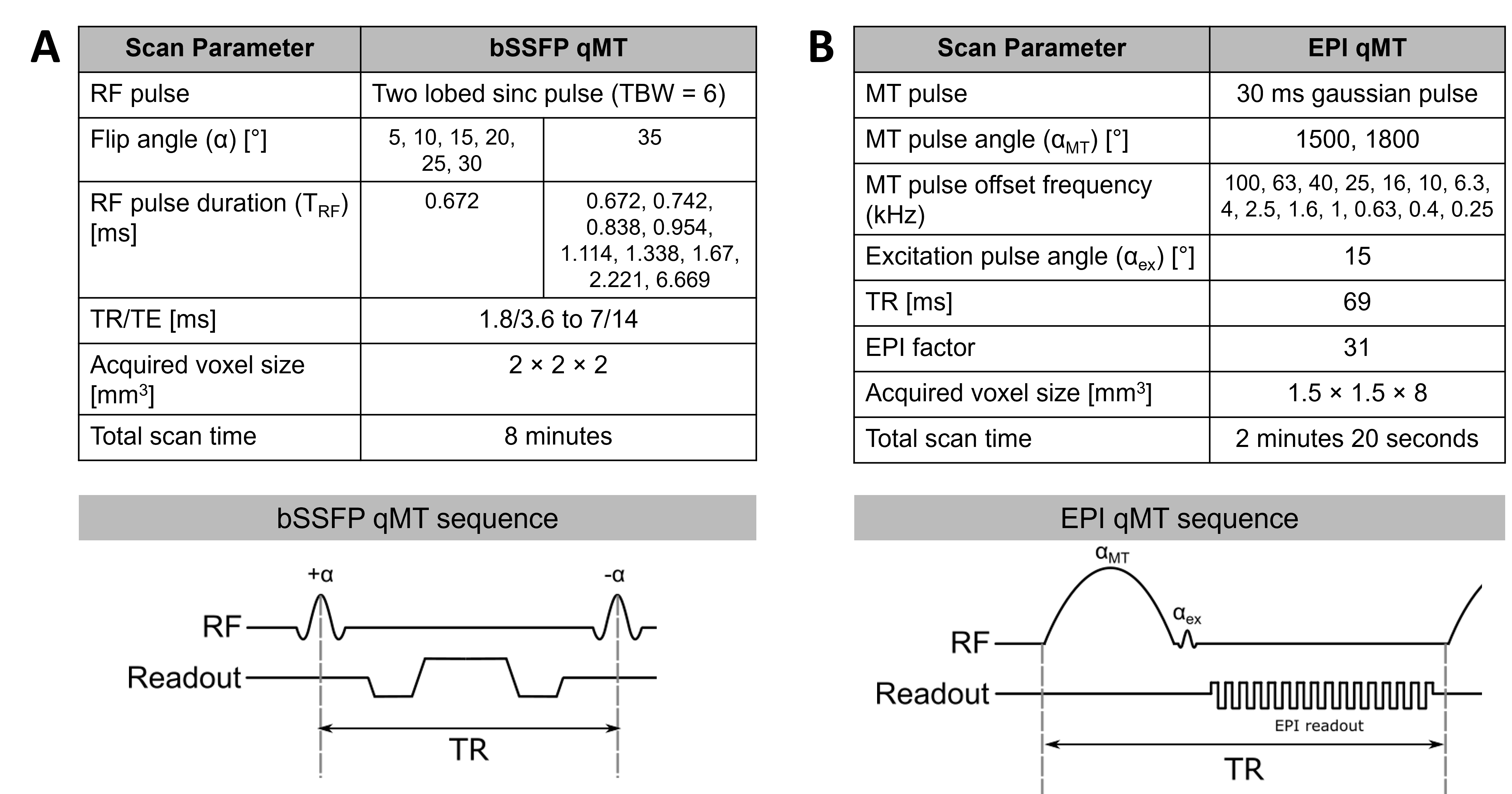
Figure 1- bSSFP & EPI qMT protocols. Scan parameters and pulse sequence components for both (A) bSSFP qMT and (B) EPI qMT protocols. For bSSFP qMT, the MT-weighting is controlled by RF excitation pulse flip angle and duration. For EPI qMT, the MT-weighting is controlled by the MT pulse offset frequency and flip angle.
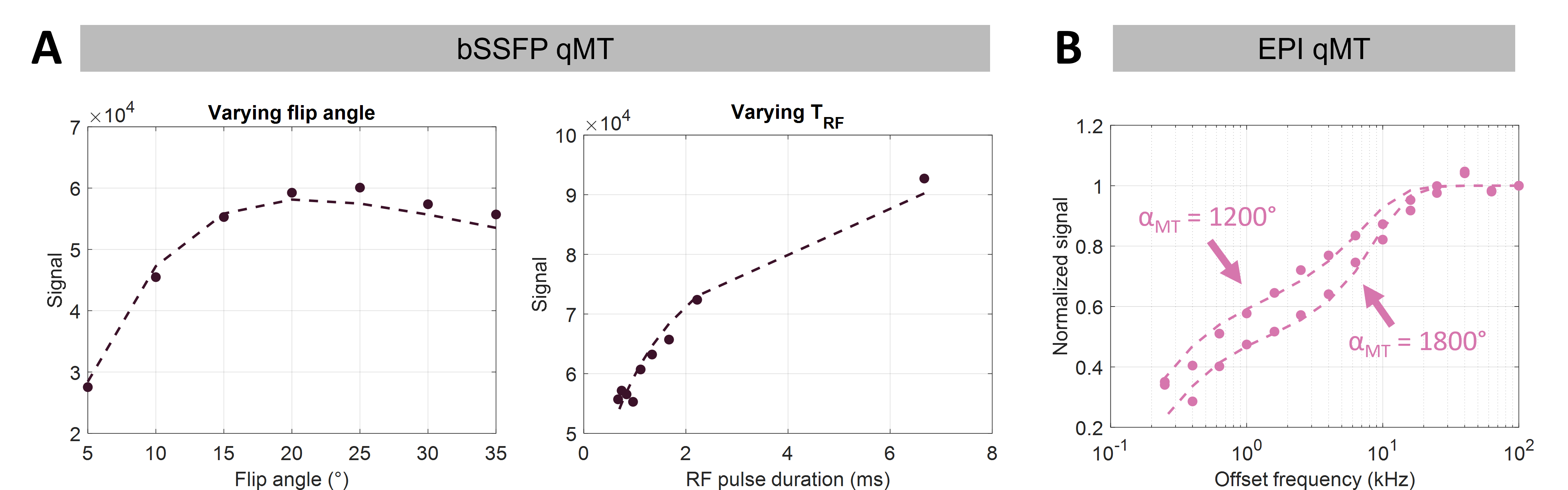
Figure 2 - Signal curves. Example white-matter signals for (A) bSSFP and (B) EPI qMT. The model (dashed lines) for each is fitted using lsqcurvefit in MATLAB. For EPI qMT, the signal was normalized to the signal at the greatest offset frequency to accelerate fitting.
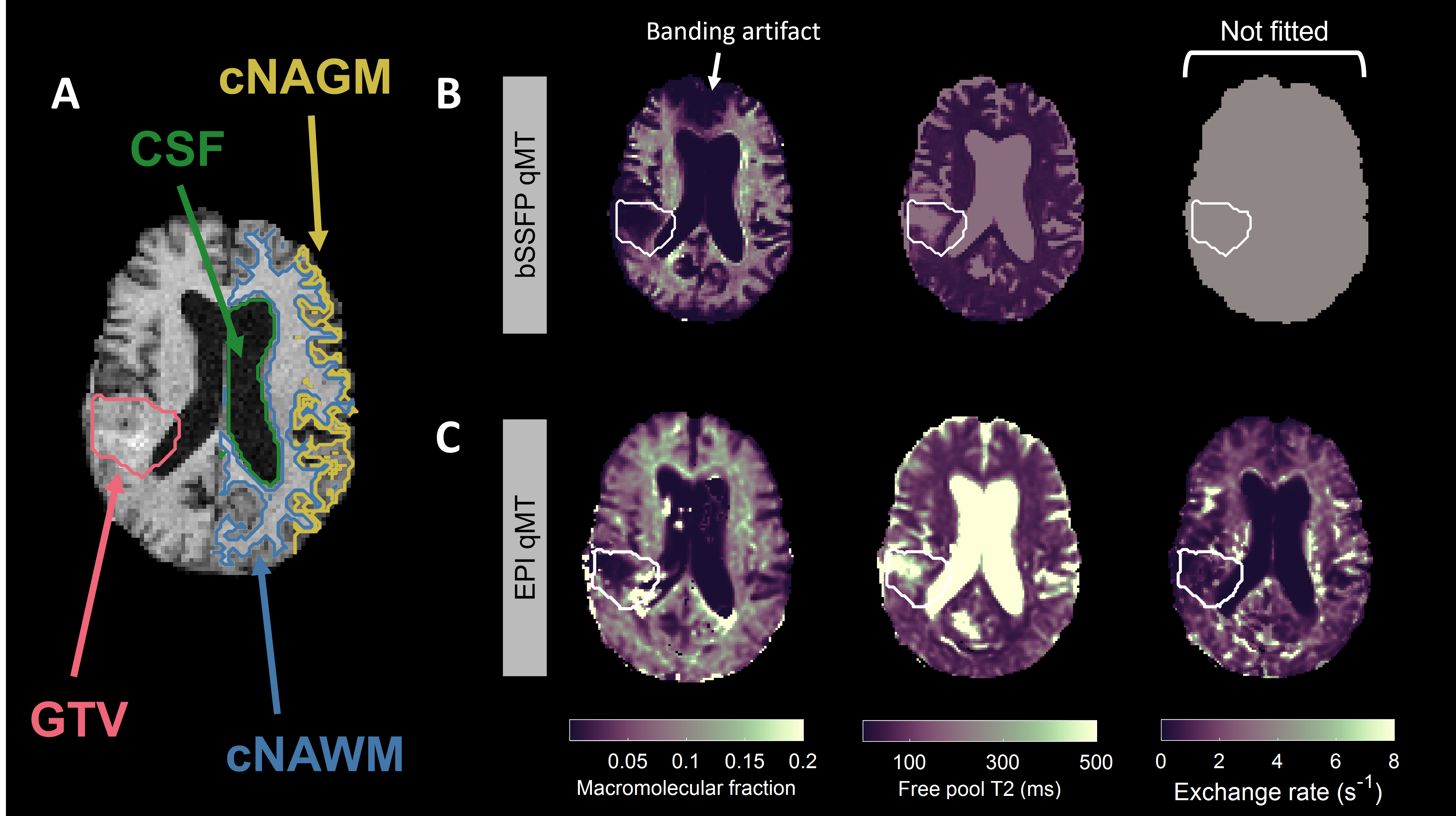
Figure 3 - ROIs and parameter maps. (A) Example ROIs are shown as contours on an anatomical T1-weighted image. Macromolecular fraction, exchange rate and free pool T2 parameter maps for both (B) bSSFP qMT and (C) EPI qMT. The maps are from the same patient for consecutive treatment fractions. The white contour is the GTV. The bSSFP map is affected by B0-banding artifacts (white arrow).
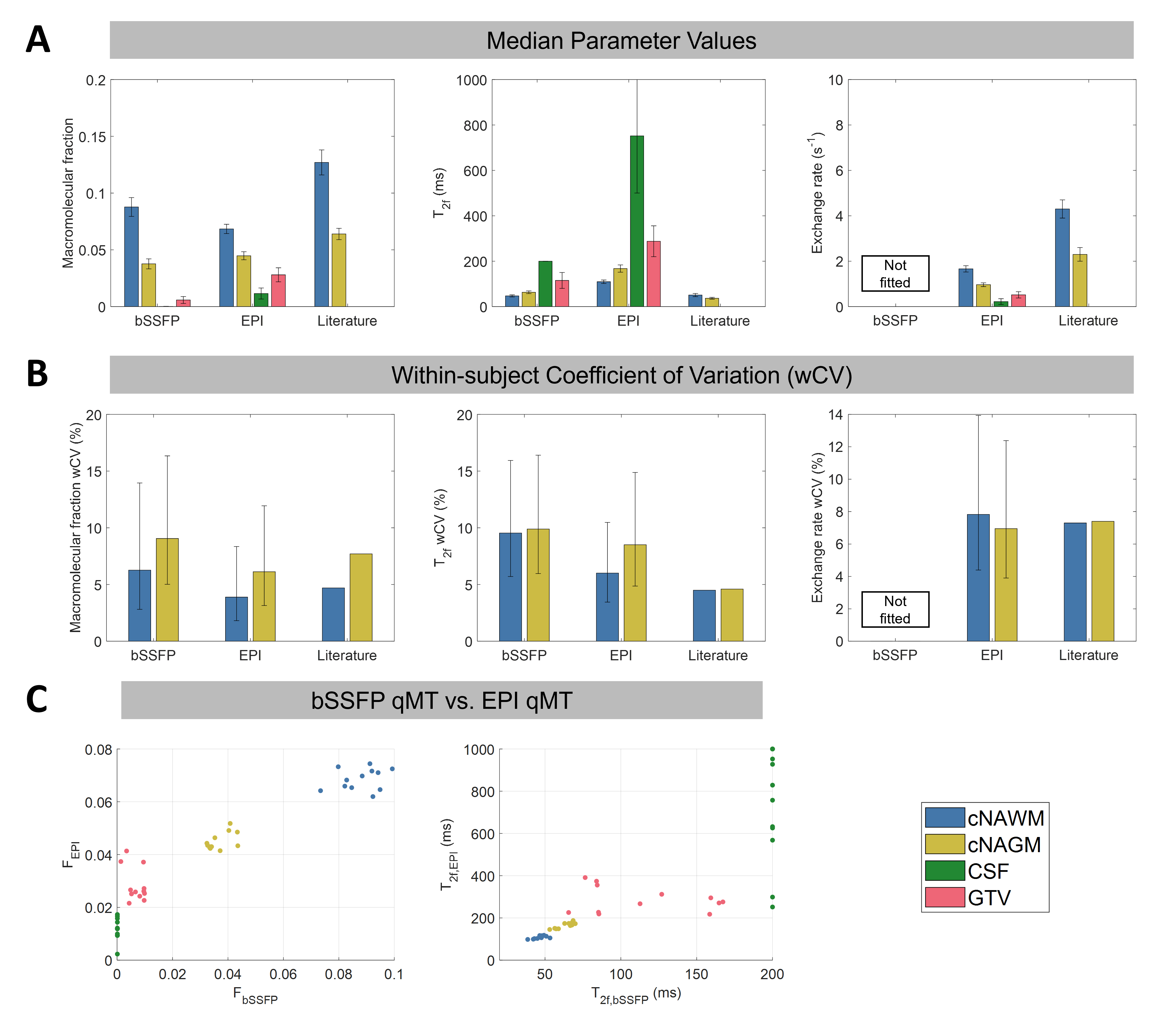
Figure 4 - ROI analysis. Median values (A), within-subject coefficient of variation (B) and scatter plots (C) are shown for each qMT parameter. Exchange rate derived from bSSFP qMT was excluded from the analysis as it was not a fitted parameter.
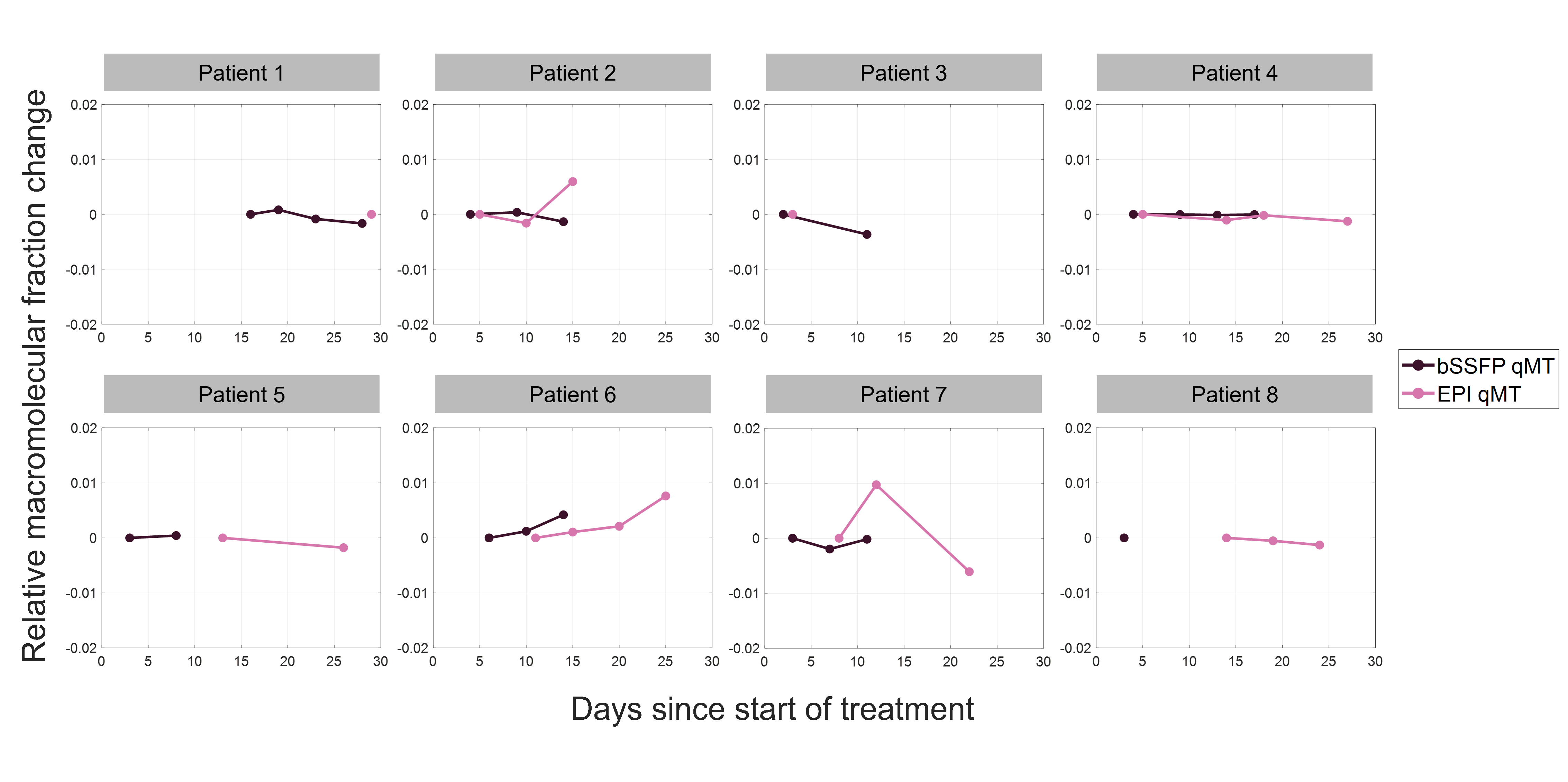
Figure 5 - Macromolecular fraction changes to the GTV. The change to macromolecular fraction in the GTV versus time during treatment is shown for both bSSFP and EPI qMT. The change is relative to the earliest image acquired for each protocol. Relative changes are larger in EPI qMT in comparison to bSSFP qMT.