4336
Frequency-Sensitive MRF (FS-MRF) for improved multi-tissue compartment modelling: a glimpse to tissue frequency from RF frequency1Department of Radiology, Stanford University, Stanford, CA, United States, 2Department of Biomedical Engineering, University of Virginia, Charlottesville, VA, United States, 3Department of Radiation Oncology, City of Hope National Cancer Center, Los Angeles, CA, United States, 4Department of Radiology and Biomedical Imaging, University of California, San Francisco, CA, United States, 5Department of Electrical Engineering, Stanford University, Stanford, CA, United States
Synopsis
Keywords: New Signal Preparation Schemes, MR Fingerprinting
Motivation: Can we encode the tissue's frequency by using RF's frequency?
Goal(s): To distinguish tissue components based on their unique frequencies.
Approach: Based on 3D MRF technique, we introduced frequency-sensitive module by varying the RF's frequency TR-to-TR.
Results: We are able to simultaneously obtain T1, T2 and frequency maps, which help improve the image fedelity and quantitative accuracy. Furthermore, it could provide a tool to differentiate the tissue components based on their frequency.
Impact: If one is interested in quantifying tissues with a frequency shift compared to water, such as fat, myelin water and some amino acids, this paper can offer a brand new angle with its noval mechanism.
Introduction
The band-limited frequency response of a typical-RF pulse enables tissues with different resonant frequencies to exhibit varied levels of RF excitation. This study aims to exploit this characteristic to distinguish tissue components based on their unique frequencies by developing a Frequency-Sensitive MRF (FS-MRF) acquisition scheme.Theory
To investigate how shifts in RF frequency influence signal evolution, we utilized a 6.0-ms hard pulse, altering its center frequency from -400Hz to +400Hz in increments of 50Hz, as depicted in Figure 1A. The resultant images, shown in Figure 1B, reveal a notably lower intensity at -150Hz. This decrease is attributable to the RF’s frequency response having a restricted energy distribution at 0Hz, which corresponds to water, as indicated by the red arrow. This results in comparable image intensities, although the image at -400Hz exhibits more pronounced fat ring artifacts compared to the +400Hz image, as expected. By employing the RF frequency response, we can encode the signal and ascertain its frequency distribution in a manner akin to MR Spectroscopic Imaging(MRSI). Nonetheless, T1 and T2 relaxation times also influence signal intensity, potentially impacting the precision of frequency estimation. To address this, we introduce frequency-sensitive MR fingerprinting as a method for simultaneous estimation of T1, T2, and frequency.Method
Sequence designThe data acquisition employed an FISP-based(1) 3D MRF(2) sequence with spiral projection trajectory(3,4), capturing data over 600 TRs for each acquisition group, with a total of 16 groups performed sequentially for comprehensive 3D k-space encoding, resulting in a net acquisition time of 8.7s per group and total time of 2 minutes and 20s for whole-brain acquisition.
The frequency-sensitive feature of the proposed FS-MRF was facilitated by varying RF frequencies of an 2.4-ms hard pulse from -300Hz to +300Hz during the 401-600TRs(Figure 2B). The shifting RF frequency allowed for tissues with identical T1/T2(800/60ms) but different frequencies(-50/0/50Hz) to take on different effective flip-angle-trains and signal evolutions(simulated using EPG(5)), shown in Figure 2C. This provides a means to differentiate and estimate tissue frequencies. In contrast, absent the RF frequency shift, the signal evolutions are similar(Figure 2D).
Reconstruction
Figure 3 shows the reconstruction pipeline, including subspace reconstruction, multi-frequency-interpolation(MFI) (4,6), and dictionary fitting.
The reconstruction outcomes can also facilitate tissue fraction segmentation by applying MRF dictionary entries with specified T1, T2, and frequency values. Notably, as the proposed method accounts for frequency effects, the segmentation of tissues with frequencies diverging from free water, such as fat(-440Hz) and myelin water(~30Hz), is rendered more accurate.
Results
Figure 4A shows the frequency, T1, and T2 maps using the proposed method. For reference, a B0 field map was procured via a dual-echo gradient-echo scan with a 1ms TE difference (4-mm resolution, 1-min scan time), and T1 and T2 maps using conventional MRF sequence. Figure 4B presents the 1st subspace coefficient map before and after B0 correction using the proposed and reference B0 maps. The red arrow points to the imprecise B0 estimation of the reference method, potentially caused by phase wrapping, leading to imperfect signal recovery in the affected regions. In contrast, our method demonstrates robustness against phase wrapping, enhancing signal recovery when combined with B0 correction. Furthermore, the conventional MRF's oversight of RF frequency response effect in reducing effective flip-angle results in inaccurate T2 estimations for fat, whereas our proposed method yields a plausible estimation(~120ms for orbital fat indicate by green arrows).Figure 5A illustrates tissue fraction maps of a brain at two distinct slices, and Figure 5B depicts the frequency, T1, and T2 maps, along with water and fat fraction maps of a thigh.
Discussion and Conclusion
Our method capitalizes on RF frequency variations to render the sequence sensitive to tissue-specific frequencies. This enables the acquisition of T1 and T2 maps, akin to traditional MRF, alongside high-resolution frequency maps. We note that the original bssfp-based MRF sequence(2) is also sensitive to frequency, but its sensitivity is detriment to the accuracy of tissue quantification at large off-resonance due to the significantly reduced signal level, which can be avoid in our FS-MRF approach. With FS-MRF, the generated frequency map is also unaffected by phase wrapping and accurately quantify tissues with significant frequency shifts, such as fat. By incorporating tissue frequency and the RF's frequency response into the signal evolution model, our method can more accurately predict the signal evolution of tissues with non-zero frequencies, thus refining the process of dictionary fitting and tissue segmentation, which offers the potential for spectrum imaging.Acknowledgements
This work was supported by: NIH research grants: R01MH116173, R01EB019437, U01EB025162, P41EB030006, R01EB033206, U24NS129893.References
1. Jiang Y, Ma D, Seiberlich N, Gulani V, Griswold MA. MR fingerprinting using fast imaging with steady state precession (FISP) with spiral readout. Magn. Reson. Med. 2015;74:1621–1631 doi: 10.1002/mrm.25559.
2. Ma D, Gulani V, Seiberlich N, et al. Magnetic resonance fingerprinting. Nature 2013;495:187–192 doi: 10.1038/nature11971.
3. Cao X, Ye H, Liao C, Li Q, He H, Zhong J. Fast 3D brain MR fingerprinting based on multi-axis spiral projection trajectory. Magn. Reson. Med. 2019;82:289–301 doi: 10.1002/mrm.27726.
4. Cao X, Liao C, Iyer SS, et al. Optimized multi‐axis spiral projection <scp>MR</scp> fingerprinting with subspace reconstruction for rapid whole‐brain high‐isotropic‐resolution quantitative imaging. Magn. Reson. Med. 2022;88:133–150 doi: 10.1002/mrm.29194.
5. Weigel M. Extended phase graphs: Dephasing, RF pulses, and echoes - Pure and simple. J. Magn. Reson. Imaging 2015;41:266–295 doi: 10.1002/jmri.24619.
6. Zhao B, Setsompop K, Adalsteinsson E, et al. Improved magnetic resonance fingerprinting reconstruction with low-rank and subspace modeling. Magn. Reson. Med. 2018;79:933–942 doi: 10.1002/mrm.26701.
7. Tamir JI, Uecker M, Chen W, et al. T2 shuffling: Sharp, multicontrast, volumetric fast spin-echo imaging. Magn. Reson. Med. 2017;77:180–195 doi: 10.1002/mrm.26102.
8. Zhang T, Pauly JM, Levesque IR. Accelerating parameter mapping with a locally low rank constraint. Magn. Reson. Med. 2015;73:655–661 doi: 10.1002/mrm.25161.
9. Ostenson J, Robison RK, Zwart NR, Welch EB. Multi-frequency interpolation in spiral magnetic resonance fingerprinting for correction of off-resonance blurring. Magn. Reson. Imaging 2017;41:63–72 doi: 10.1016/j.mri.2017.07.004.
Figures
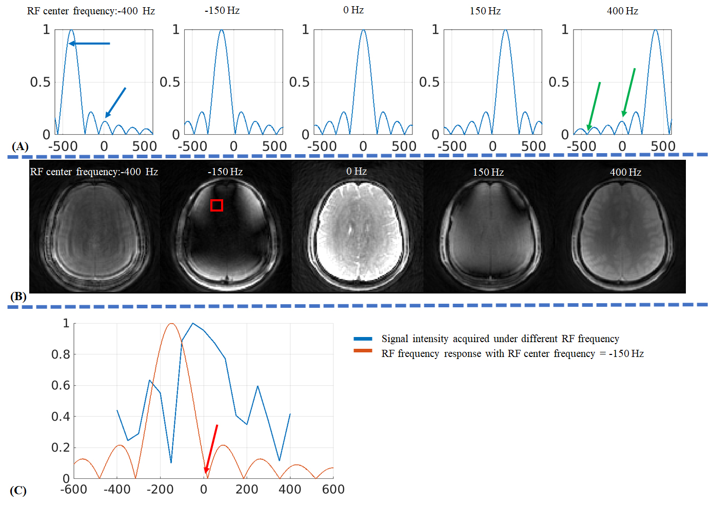
(A) The frequency response of RF shifting from -400Hz to +400Hz.
(B) The image acquired with RF frequency of -400Hz, -150Hz, 0Hz, 150Hz and 400Hz, respectively. While the -400Hz and +400Hz frequencies display identical energy distributions at 0Hz, their energy distributions at -440Hz—the primary fat frequency at 3T—are markedly different, as shown by the blue and green arrows.
(C) The signal intensity at red box region in (B) across different RF frequencies (blue line) and the RF frequency response with a -150Hz shift (red line).
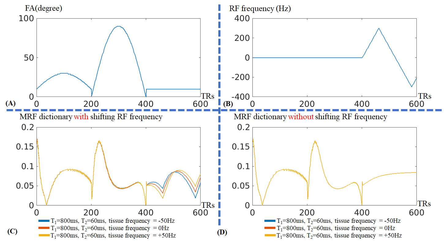
(A) Flip angle pattern.
(B) RF frequency shift pattern.
(C) Simulated signal evolutions of same T1/T2 and different tissue frequency, based on given flip angle pattern (A) and RF frequency pattern (B).
(D) Simulated signal evolutions when turn off the RF frequency shift (keep to 0Hz).
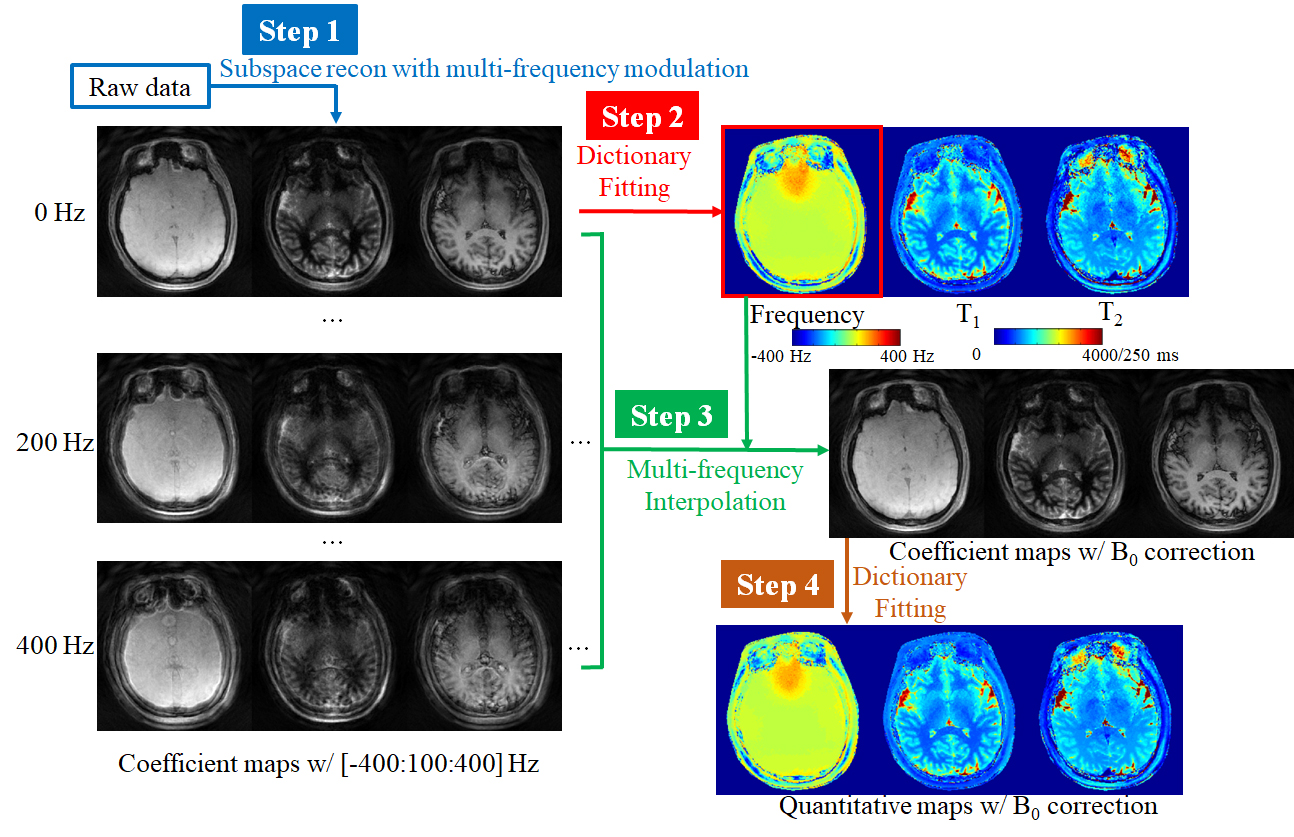
Step 1: Data undergo subspace reconstruction with a locally low-rank constraint to create subspace coefficient maps, applying MFI with phase modulation of -400Hz to +400Hz.
Step 2: Initial frequency maps are derived from the 0-Hz coefficient maps through dictionary fitting.
Step 3: These frequency maps are integrated with all multi-frequency coefficient maps for B0 correction using MFI, yielding B0-corrected coefficient maps.
Step 4: B0-corrected T1, T2, and frequency maps are obtained via dictionary fitting. Steps 2-4 may be iteratively performed to enhance image fidelity.
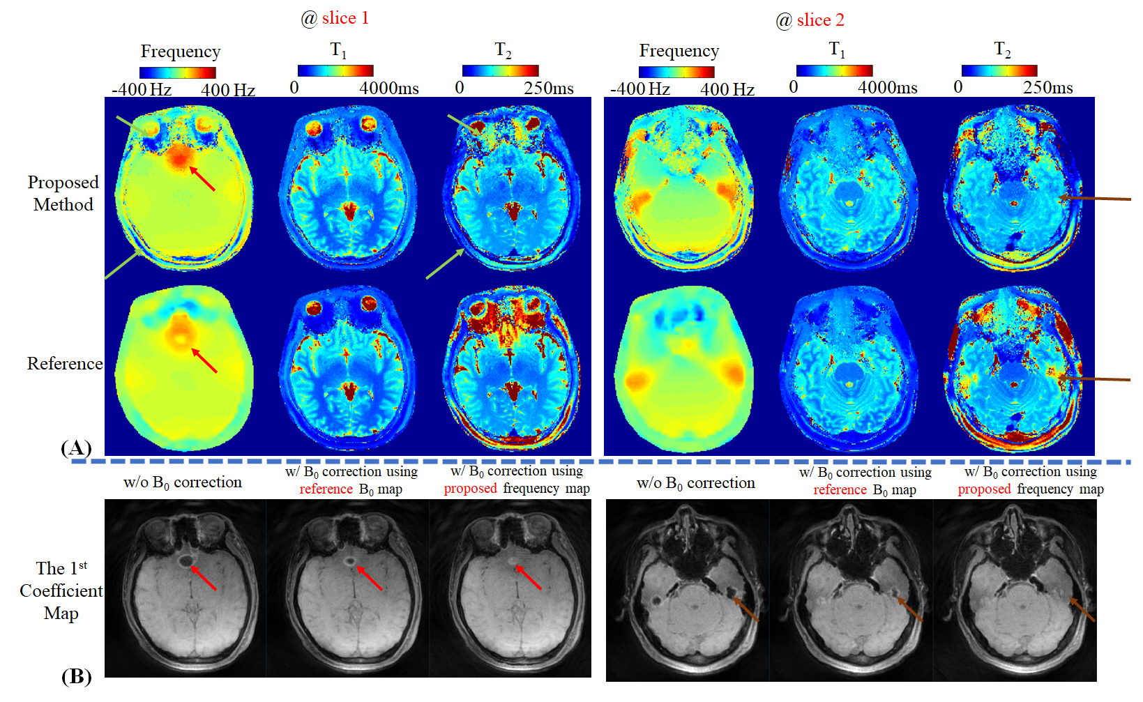
(A) The frequency, T1 and T2 maps using proposed method and reference method of two different slices in brain.
(B) shows the 1st subspace coefficient map without/with B0 correction using proposed/reference B0 maps. B0 correction using the proposed frequency maps covered more signal than that using reference B0 maps, as indicated by red and brown arrows.
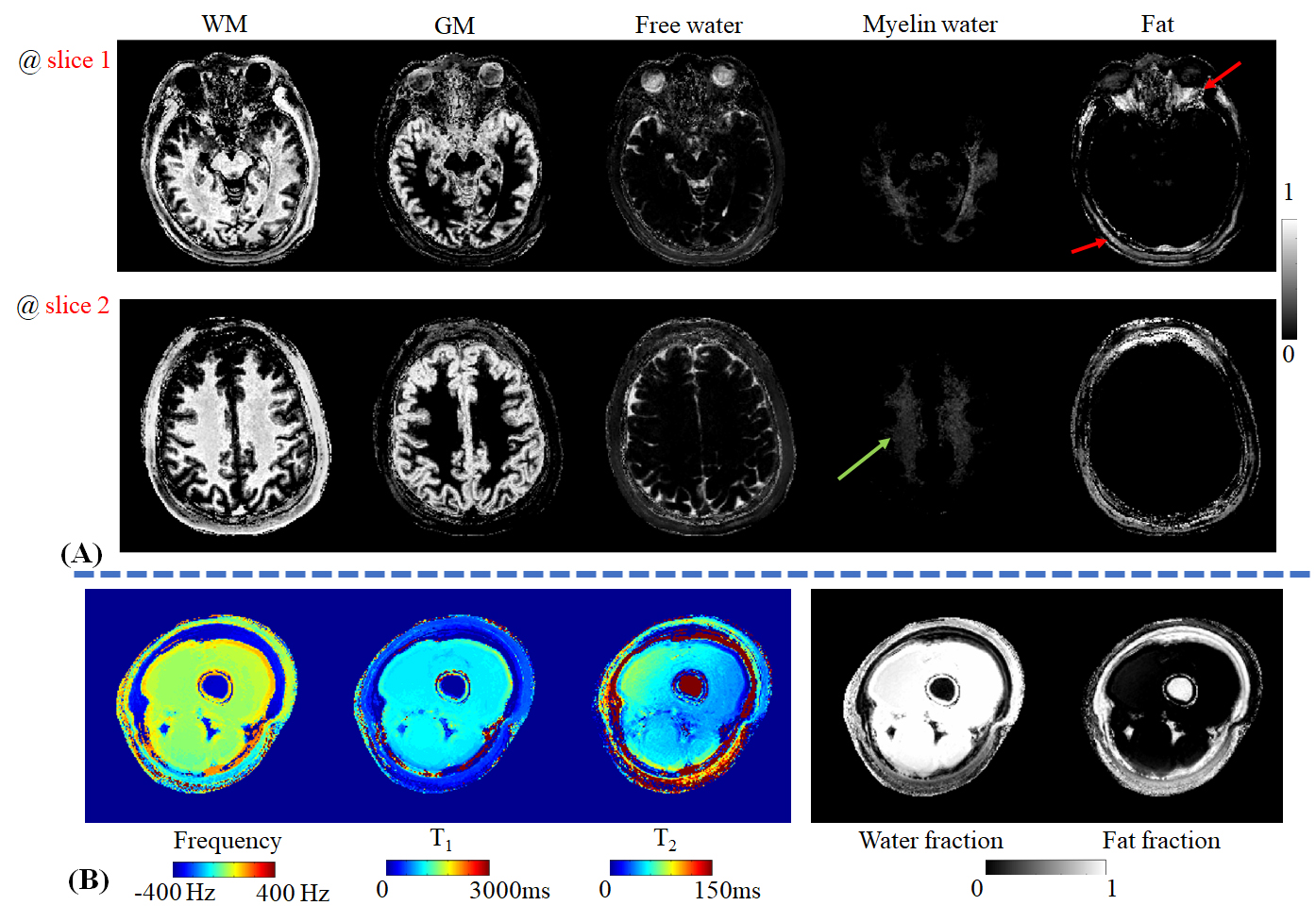
(A) Tissue fractions maps of a brain at two different slices. The red arrow indicates the orbital fat components.
(B) The frequency, T1 and T2 maps as well as water and fat fraction maps.