4108
Susceptibility tensor imaging of ex vivo human hemibrain using 7T human MR scanner1Department of Radiology, Johns Hopkins University, Baltimore, MD, United States, 2F.M. Kirby Research Center for Functional Brain Imaging, Kennedy Krieger Institute, Baltimore, MD, United States, 3Department of Pathology, Johns Hopkins University, Baltimore, MD, United States, 4The Richman Family Precision Medicine Center of Excellence in Alzheimer's Disease, Baltimore, MD, United States
Synopsis
Keywords: Preclinical Image Analysis, Microstructure
Motivation: High-resolution ex vivo susceptibility tensor imaging (STI) shows promise in visualizing detailed microstructural neuroanatomy related to tissue magnetic susceptibility contrast but is usually challenging with large human brain samples.
Goal(s): This work aimed to demonstrate a feasible protocol for STI on postmortem human hemibrain using a 7T human MR scanner.
Approach: De-identified human brain samples of the left hemisphere were collected, prepared, and scanned with a 3D multi-echo gradient echo sequence with 0.5 mm isotropic resolution.
Results: Multi-orientation quantitative susceptibility mapping and STI with a maximum of 12 orientations were obtained. Myelinated fibers and iron deposition in cortical substructures were visualized.
Impact: The proposed ex vivo MRI protocol is expected to be helpful to researchers interested in STI. The ex vivo STI acquired through this protocol may provide anatomical references for in vivo STI studies.
INTRODUCTION
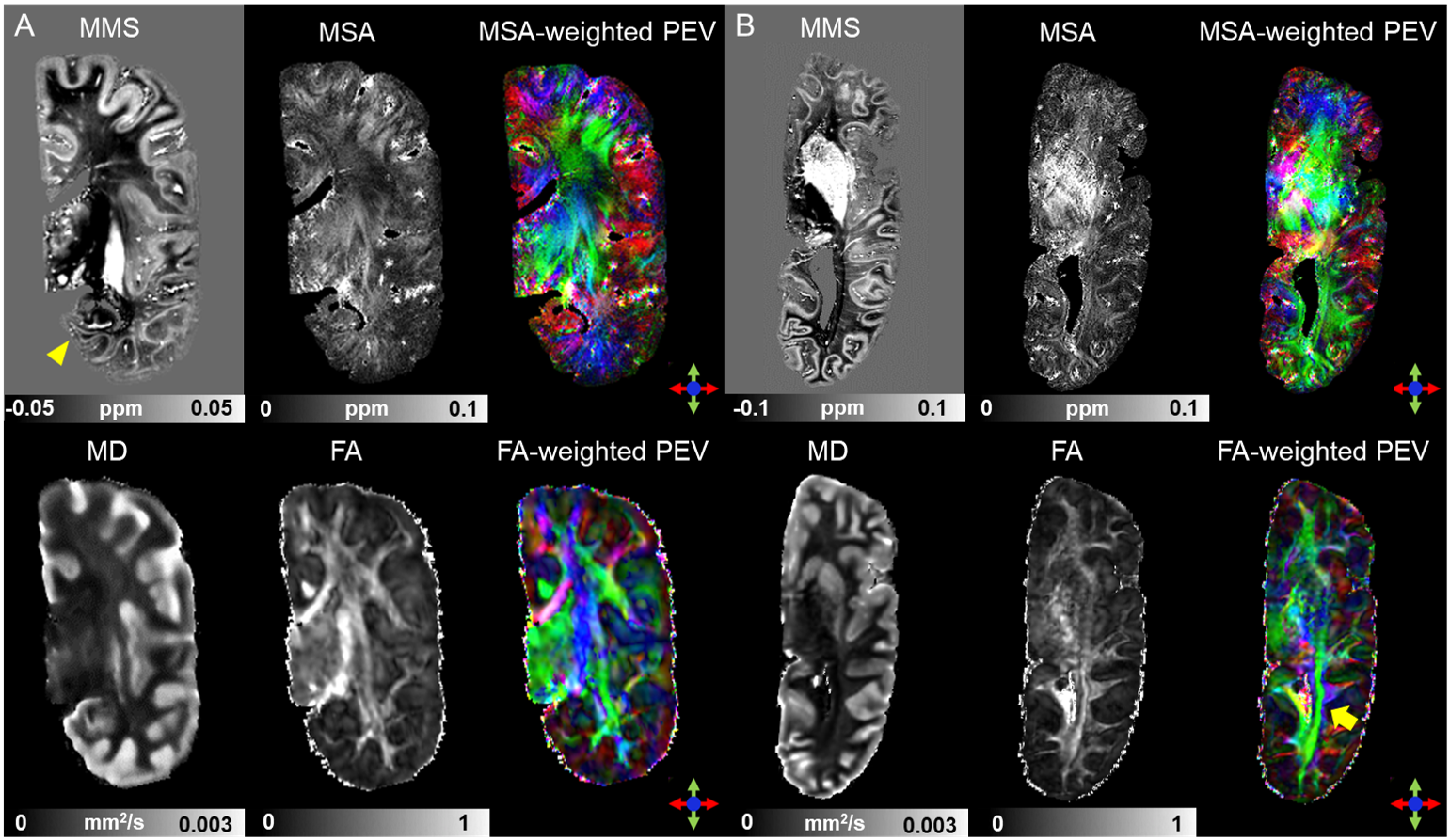
Susceptibility tensor imaging (STI) aims at quantifying anisotropic tissue magnetic susceptibility from MR phase measures acquired at multiple sample orientations relative to the main magnetic field (B0) using a second-order tensor model1-3. High-resolution STI metrics, such as mean magnetic susceptibility (MMS), magnetic susceptibility anisotropy (MSA), and MSA-weighted principal eigenvector (PEV) maps, show promise in visualizing detailed microstructural neuroanatomy related to tissue magnetic susceptibility contrast3-5. Here, we aimed to test a STI scan protocol with 0.5 mm isotropic resolution using postmortem human hemibrains on a human 7T MRI scanner (Philips Healthcare, Best, the Netherlands).MATERIALS AND METHODS
Brain sampleDe-identified postmortem hemibrains of the left hemisphere were provided by the Johns Hopkins Brain Resource Center. At autopsy, the fresh brains weighed within the normal ranges and gross examinations revealed no abnormal findings. The hemibrains were fixed in 10% formaldehyde for more than 3 months before the preparation for ex vivo MRI scans to ensure complete fixation of the entire sample as performed in previous studies5, 6.
Designing and creating the rotatable ellipsoid-shaped container
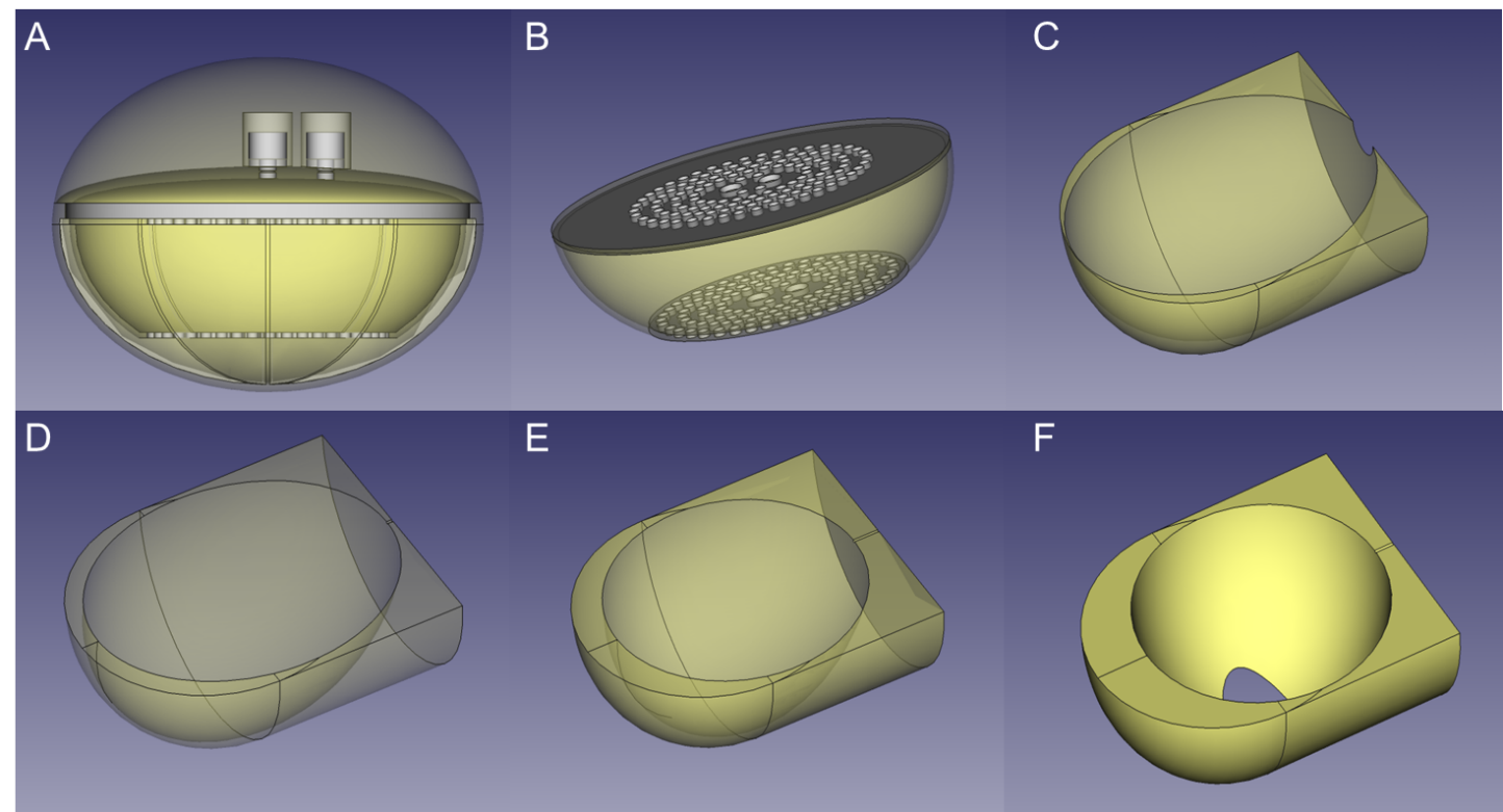
To facilitate MRI scans for the hemibrain at multi-orientations along the x (right-left) and y (anterior-posterior) axes, a rotatable ellipsoid-shaped container was designed to hold the sample tightly. The container was 3D printed for an ellipsoidal shape with two equal radii of 87 mm and one larger radius of 112 mm (Figure 1). Four bases were also 3D printed to hold the container at different angles around the x-axis.
Pre-imaging steps
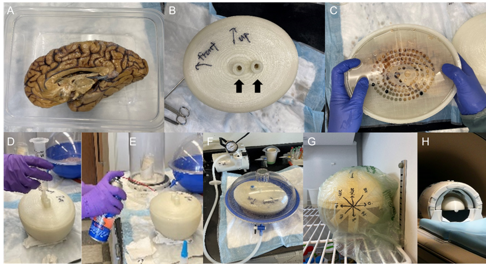
A set of procedures for the sample preparation from formalin fixation to MRI scan is summarized (Figure 2).
MRI scans
3D multi-echo GRE sequence was acquired at 7T: repetition time (TR)/echo time (TE)/ΔTE = 47/3/4 ms, 5 unipolar echoes, flip angle = 12°, field of view (FOV) = 224 × 180 × 90 mm3, 0.5 mm isotropic resolution, bandwidth = 502 Hz/voxel, SENSE factor of 2 × 2, scan time = 17 min 46 s per orientation. For STI, GRE scans using the same protocol were collected at 12 different brain orientations relative to the B0 field. For comparison with diffusion tensor imaging (DTI), diffusion MRI was acquired at 3T with a multi-shot EPI sequence: TR/TE=12500/81 ms, FOV =224 × 128 × 72 mm3, 1.5 mm isotropic resolution, EPI factor of 21, 2 shells with b-values to be 5000 and 10000 s/mm2 with 24 diffusion weighting directions per shell, scan time = 4 h 3 min. Diffusion MRI with reversed phase encoding (FH/HF) was also acquired.
Data processing
Phase images were preprocessed using best-path based phase unwrapping7, weighted averaging for echo combination8, and VSHARP for background field removal with maximum SMV kernel size of 6 mm9, 10. Preprocessed phase images at different orientations were nonlinearly co-registered to the reference position using ANTs11. Qualitative susceptibility mapping (QSM) using COSMOS12 was then calculated with reference to the whole brain susceptibitliy. MMS, MSA, and MSA-weighted PEV maps were calculated using asymmetric STI approach without explicit regularization13. Diffusion MRI was processed using Tortoise 4.014 and MRtrix315 to calculate mean diffusivity (MD), fractional anisotropy (FA), and FA-weighted PEV maps and co-registered to STI space.
RESULTS
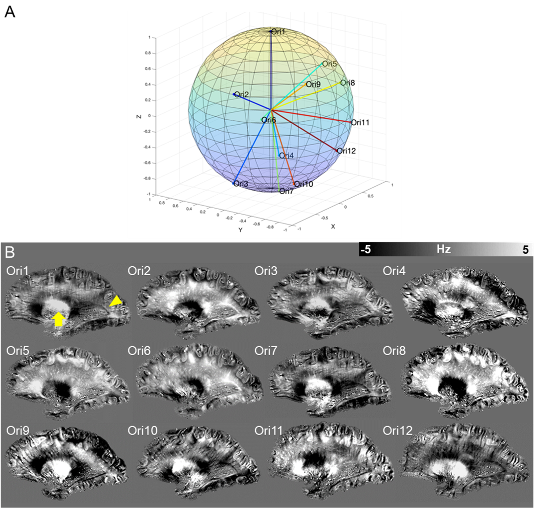
Orientation dependence of GRE tissue frequency map (Figure 3)For co-registered GRE scans, unit vectors of the B0 field in the subject frame of reference spanned uniformly across a half-spherical surface (Figure 3A). Tissue frequency maps demonstrated large orientation dependence across the brain, especially around the basal ganglia and the major white matter fiber bundles (Figure 3B).
Anatomical identification on QSM (Figure 4)
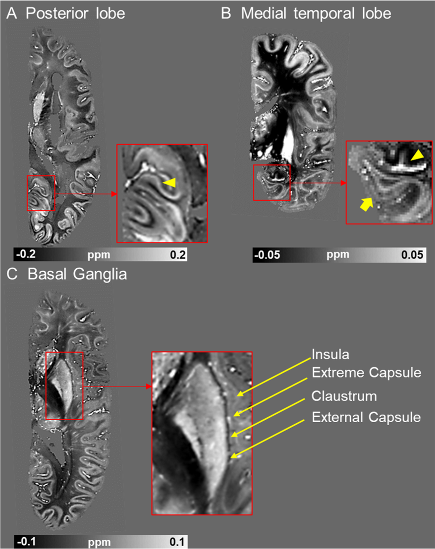
The lines of Gennari within the visual cortex around the calcarine fissure (Figure 4A), cortical substructures in the hippocampus and entorhinal cortex (Figure 4B), and detailed structures around the basal ganglia could be visualized (Figure 4C).
Comparison between STI and DTI (Figure 5)
The cortical substructures in the medial temporal lobe could be seen in the high-resolution MMS (Figure 5A). The MSA-weighted PEV in STI showed limited consistency with the FA-weighted PEV in DTI (Figure 5B).
DISCUSSION
Our ex vivo human brain STI protocol was useful for the visualization of microstructural neuroanatomy as well as the accumulation of postmortem human GRE data for future training and validation of data-driven STI reconstructions with sparse orientation sampling16, 17. Discrepancies between the PEV derived from STI and that from DTI might partly come from the enhanced chemical exchange effect and reduced susceptibility anisotropy due to fixation18.CONCLUSION
We have demonstrated a feasible ex vivo STI protocol to scan human hemibrain at multiple orientations. Fine microstructural details in the neuroanatomy of the human brain can be visualized using the obtained QSM and STI data.Acknowledgements
This work is supported by NIH NIBIB (P41EB031771), the Richman Family Precision Medicine Center of Excellence in Alzheimer's Disease including significant contributions from the Richman Family Foundation, the Rick Sharp Alzheimer’s Foundation, the Sharp Family Foundation and others. Kenichi Oishi is a consultant for “AnatomyWorks” and “Corporate-M.” Peter van Zijl has research support from and technology licensed to Philips Healthcare and has also been a paid speaker. This arrangement is being managed by the Johns Hopkins University in accordance with its conflict-of-interest policies. The authors thank the Brain Resource Center for providing the brain specimens and Mary McAllister for English-language editing.
References
References
1. Liu C. Susceptibility tensor imaging. Magn Reson Med 2010;63:1471-1477.
2. Li W, Wu B, Avram AV, Liu C. Magnetic susceptibility anisotropy of human brain in vivo and its molecular underpinnings. Neuroimage 2012;59:2088-2097.
3. Li X, Vikram DS, Lim IA, et al. Mapping magnetic susceptibility anisotropies of white matter in vivo in the human brain at 7 T. Neuroimage 2012;62:314-330.
4. Liu C, Li W, Wu B, et al. 3D fiber tractography with susceptibility tensor imaging. Neuroimage 2012;59:1290-1298.
5. Li W, Liu C, Duong TQ, et al. Susceptibility tensor imaging (STI) of the brain. NMR Biomed 2017;30.
6. Dawe RJ, Bennett DA, Schneider JA, et al. Postmortem MRI of human brain hemispheres: T2 relaxation times during formaldehyde fixation. Magn Reson Med 2009;61:810-818.
7. Shatil AS, Uddin MN, Matsuda KM, Figley CR. Quantitative Ex Vivo MRI Changes due to Progressive Formalin Fixation in Whole Human Brain Specimens: Longitudinal Characterization of Diffusion, Relaxometry, and Myelin Water Fraction Measurements at 3T. Front Med (Lausanne) 2018;5:31.
8. Abdul-Rahman HS, Gdeisat MA, Burton DR, et al. Fast and robust three-dimensional best path phase unwrapping algorithm. Appl Opt 2007;46:6623-6635.
9. Wu B, Li W, Avram AV, et al. Fast and tissue-optimized mapping of magnetic susceptibility and T2* with multi-echo and multi-shot spirals. Neuroimage 2012;59:297-305.
10. Schweser F, Deistung A, Lehr BW, Reichenbach JR. Quantitative imaging of intrinsic magnetic tissue properties using MRI signal phase: an approach to in vivo brain iron metabolism? Neuroimage 2011;54:2789-2807.
11. Wu B, Li W, Guidon A, Liu C. Whole brain susceptibility mapping using compressed sensing. Magn Reson Med 2012;67:137-147.
12. Tustison NJ, Cook PA, Holbrook AJ, et al. The ANTsX ecosystem for quantitative biological and medical imaging. Sci Rep 2021;11:9068.
13. Liu T, Spincemaille P, de Rochefort L, et al. Calculation of susceptibility through multiple orientation sampling (COSMOS): a method for conditioning the inverse problem from measured magnetic field map to susceptibility source image in MRI. Magn Reson Med 2009;61:196-204.
14. Cao S, Wei H, Chen J, Liu C. Asymmetric susceptibility tensor imaging. Magn Reson Med 2021;86:2266-2275.
15. Irfanoglu MO, Modi P, Nayak A, et al. DR-BUDDI (Diffeomorphic Registration for Blip-Up blip-Down Diffusion Imaging) method for correcting echo planar imaging distortions. Neuroimage 2015;106:284-299.
16. Tournier JD, Smith R, Raffelt D, et al. MRtrix3: A fast, flexible and open software framework for medical image processing and visualisation. Neuroimage 2019;202:116137.
17. Bao L, Xiong C, Wei W, et al. Diffusion-regularized susceptibility tensor imaging (DRSTI) of tissue microstructures in the human brain. Med Image Anal 2021;67:101827.
18. Fang Z, Lai KW, van Zijl P, et al. DeepSTI: Towards tensor reconstruction using fewer orientations in susceptibility tensor imaging. Med Image Anal 2023;87:102829.
19. Chan
KS, Hédouin R, Mollink J, et al. Imaging white matter microstructure with
gradient-echo phase imaging: Is ex vivo imaging with formalin-fixed tissue a
good approximation of the in vivo brain? Magn Reson Med 2022;88:380-390.
Figures