4077
A comparison study of different eddy current measurements at low field portable MRI1School of Biomedical Engineering, Shanghai Jiao Tong University, Shanghai, China, 2National Engineering Research Center of Advanced Magnetic Resonance Technologies for Diagnosis and Therapy (NERC-AMRT), Shanghai Jiao Tong University, Shanghai, China, 3Wuxi Marvel Stone Healthcare Co. Ltd., Wuxi, China
Synopsis
Keywords: Low-Field MRI, Low-Field MRI, eddy current measurement, field probe
Motivation: Eddy current results in resolution degradation and unwanted phase variations. However, there have been relatively few eddy-current related studies carried out in low field recently.
Goal(s): Our goal was to introduce and compare image-phase based and FID-phase based eddy current measurement techniques in a 64mT MRI system and reduced eddy-current effects.
Approach: We employed a large phantom or six field probes to measure eddy-current-induced gradients shift. And we modeled them as sums of exponentially decaying components to compensate the gradient unit.
Results: Eddy-current-induced field shift was initially about 350ppm, and reduced to 240ppm and 20ppm by these two methods.
Impact: This work develops two methods for measuring eddy current in low-field MRI, especially for portable scanner, which help reducing eddy-current-induced effects and improving the image quality of clinical sequence (e.g. DWI, DTI) in low field scanner.
Introduction
Eddy current is induced by the application of gradient pulses, and results in extra gradients and B0 shift, generating undesired intensity and phase variations which produce artifacts and distortion1. In low-field MRI, some commonly used fast acquisition sequences, such as EPI, is significant for the development of clinical applications2. Also, some correction methods have high requirements for phase accuracy under such low SNR (e.g. TOPUP). However, in permanent magnets under low field strength, especially portable MRI, works on eddy currents measurement and compensation have not been developed well as high-field.In this work, we introduced two eddy current measurement techniques3, 4 in a permanent 64mT low-field MRI system. One was based on the image phase from a large symmetrical phantom without additional hardware equipment. The other was based on the FID phase from a six-point field probe device, which had higher acquisition accuracy and efficiency since it allowed for simultaneous on-axis and cross terms. We successfully modeled first-order eddy-current-induced gradient terms and compensated the gradient unit by these two methods. Finally, the impact of eddy current was reduced by one order of magnitude.
Methods
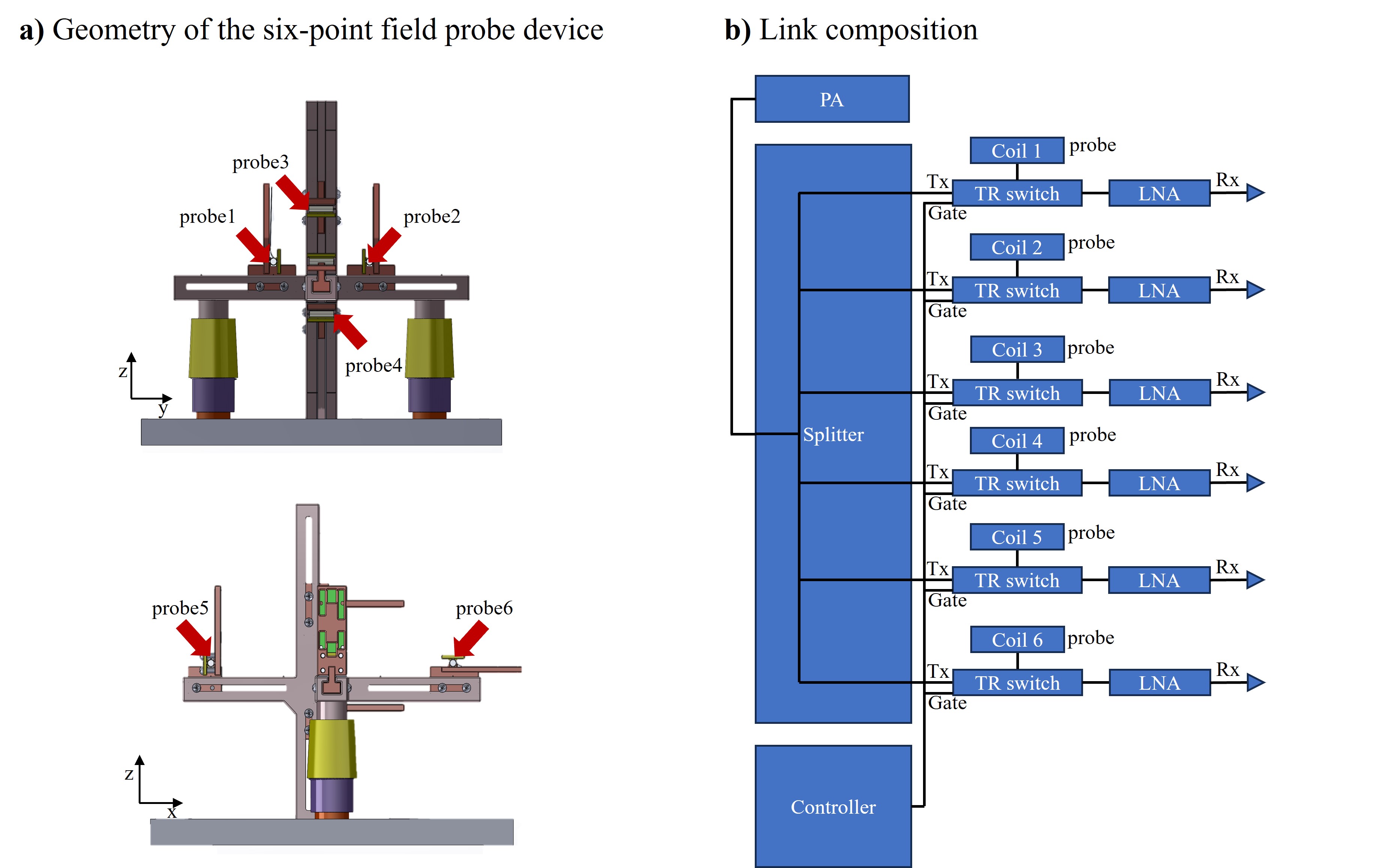
Hardware set upIn the first method, we used a spherical phantom with a diameter of 150mm, without extra hardware. For comparison, we developed a six-point active TX/RX field probe device as shown in Figure 1a. To compensate the poor SNR in low-field MRI, each probe consisted of a 20mm x 3.5mm (inner diameter) CuSO4 doped water cylinder phantom with short T1. The probes were symmetrically distributed in groups of two on three axes so as to fit the first-order eddy current model more easily. The placement positions were able to be adjusted from ±40mm to ±100mm along their belonging axes. Splitters and TR switches were required in the second method (Figure 1b).
Experiments set up
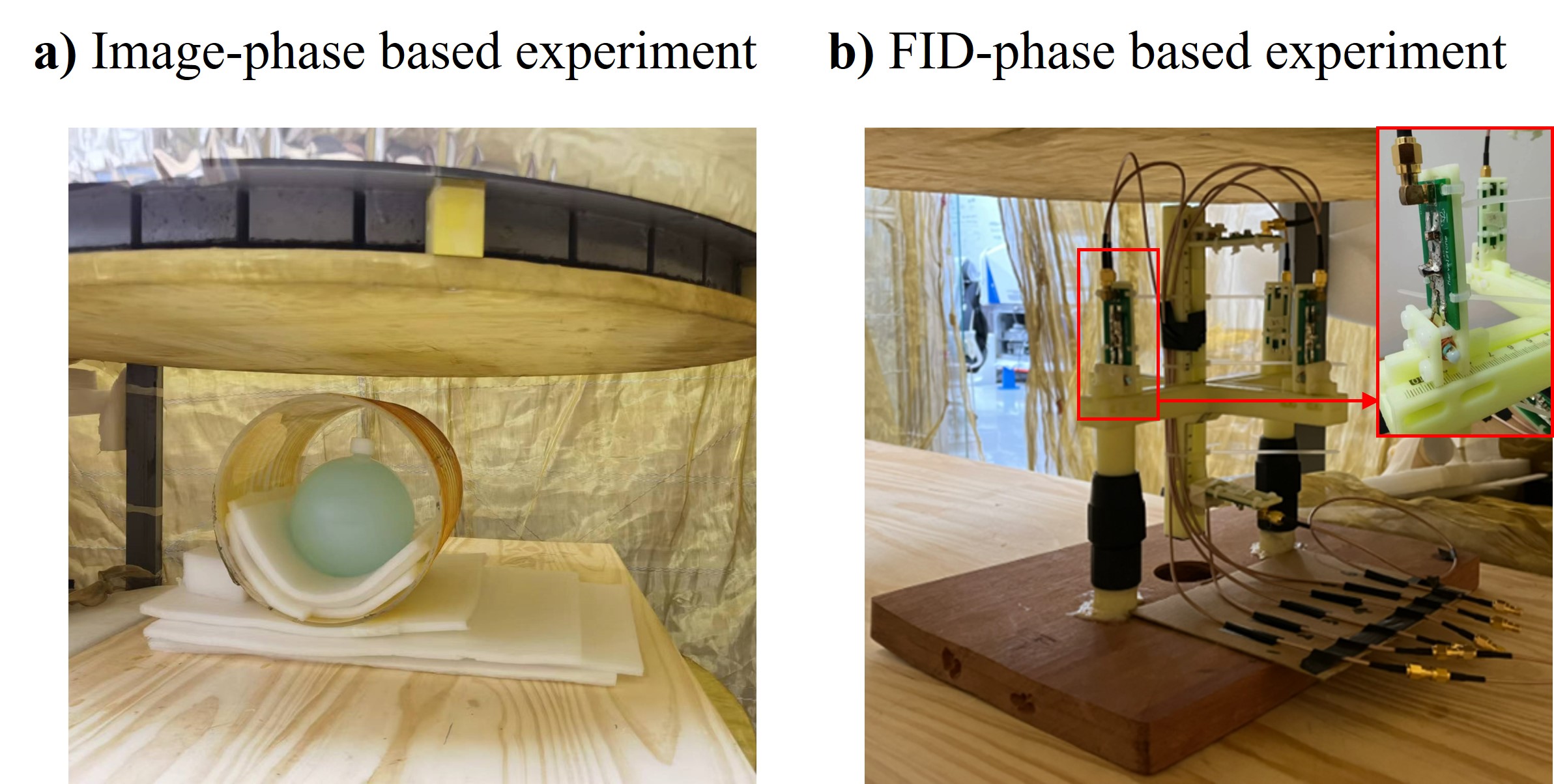
The pulse sequence consisted of a long-duration gradient pulse of positive or negative polarity followed by a RF excitation pulse and a variable delay time. The total acquisition time of the image-phase based method is about six to seven times that of the FID-phase method. Two measurement devices were placed in the center of the magnetic field as shown in Figure 2.
Mechanism
Both two methods are based on calculating the phase difference between the signal we gain after the gradient pulse Gtest of positive and negative polarity. The signal we gain from the 1-D projection of the large phantom is5:
$$\phi_+(r,t)=\gamma\int_{0}^{t} (G_r\cdot r+G_e(r,\tau)\cdot r+B_e(\tau))d\tau +\phi_0 (1)$$
$$ \phi_-(r,t)=\gamma\int_{0}^{t} (G_r\cdot r+G_e( r,\tau)\cdot r+B_e(\tau))d\tau +\phi_0 (2)$$
where $$$\phi_+$$$ and $$$\phi_-$$$ represent the total phase signal and $$$G_r$$$ is the readout gradient in order to encode the location information along one direction. $$$G_e$$$ and $$$B_e$$$ represent the extra signal resulting from the eddy current. Different from the first image-phase based method, six-point field probe device collects FID signal of each small phantom. The FIDs also include the $$$G_e$$$ and $$$B_e$$$.
Data analysis
The time-dependent data we gather by either the large phantom or field probe can be modeled as sum of several exponentially decaying components with independent amplitudes $$$A_i$$$ and time constants $$$\tau_i$$$6, 7 :
$$y(t)=G\sum_{i=1}^m A_ie^{-\frac{t}{\tau_i}} (3)$$
where $$$y(t)$$$ can be considered as $$$G_e$$$ or $$$B_e$$$. m here we use is 6, which is related to the eddy current model accuracy and eddy current compensation capability of the MR system.
Results and Discussion
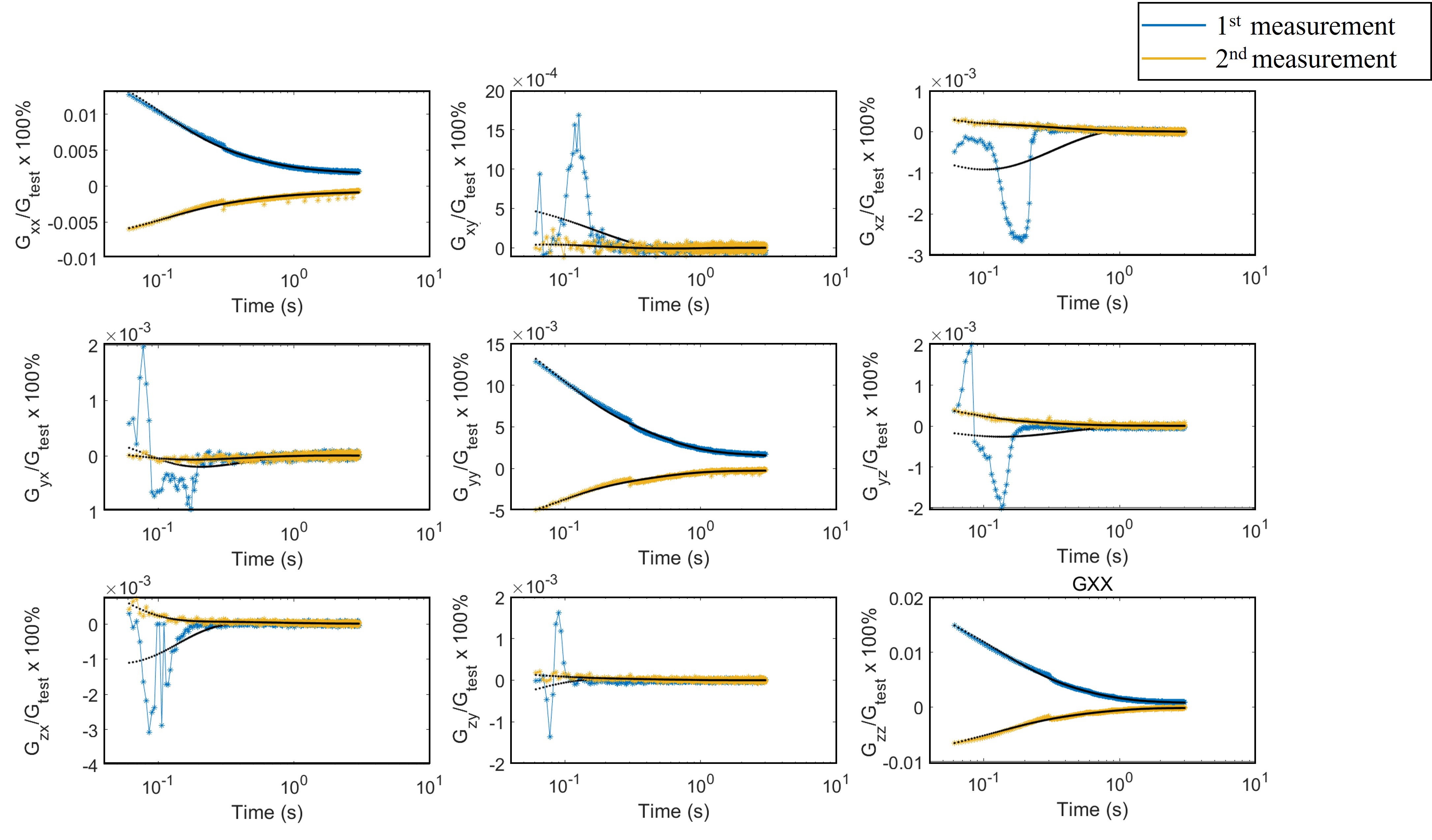
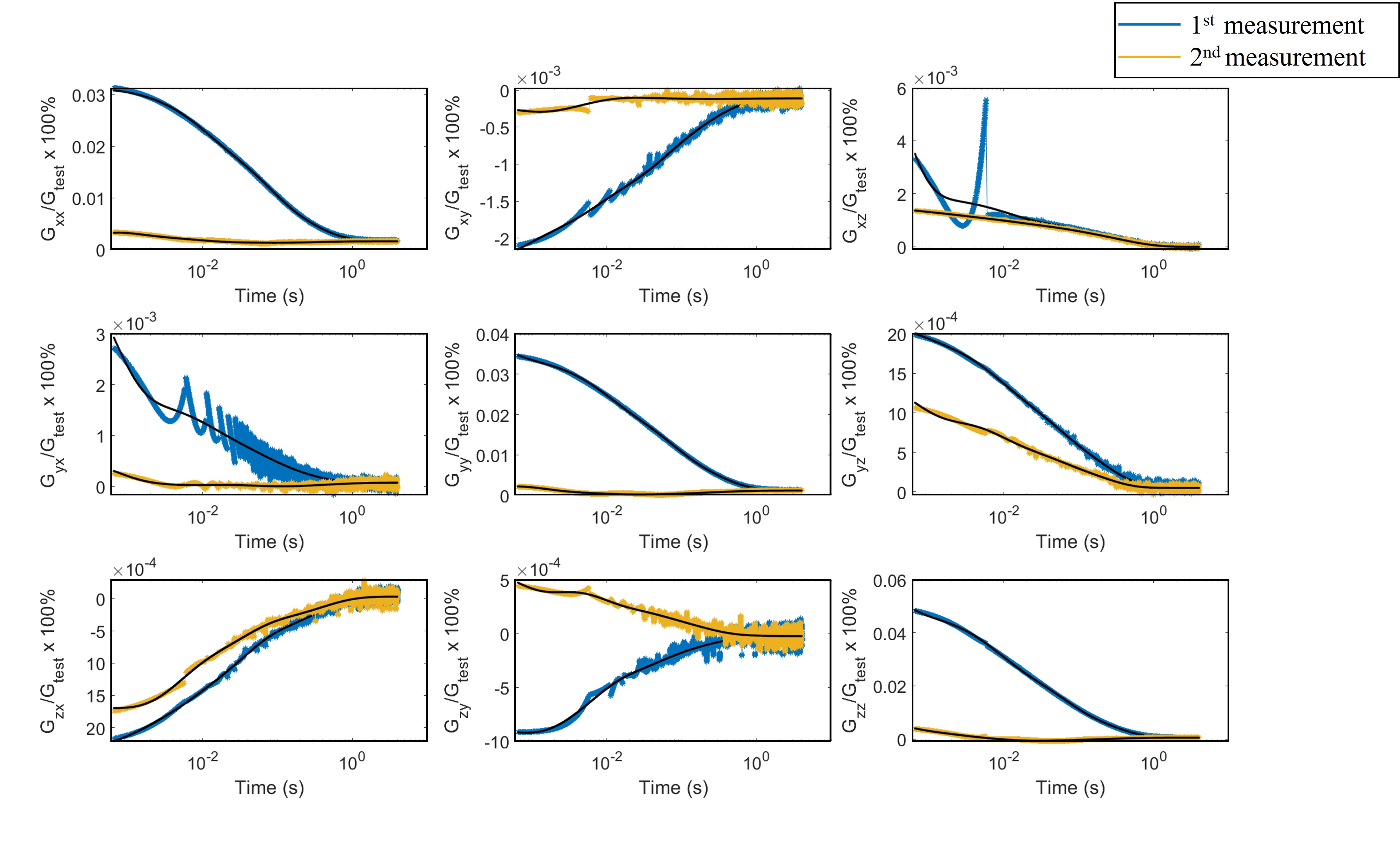
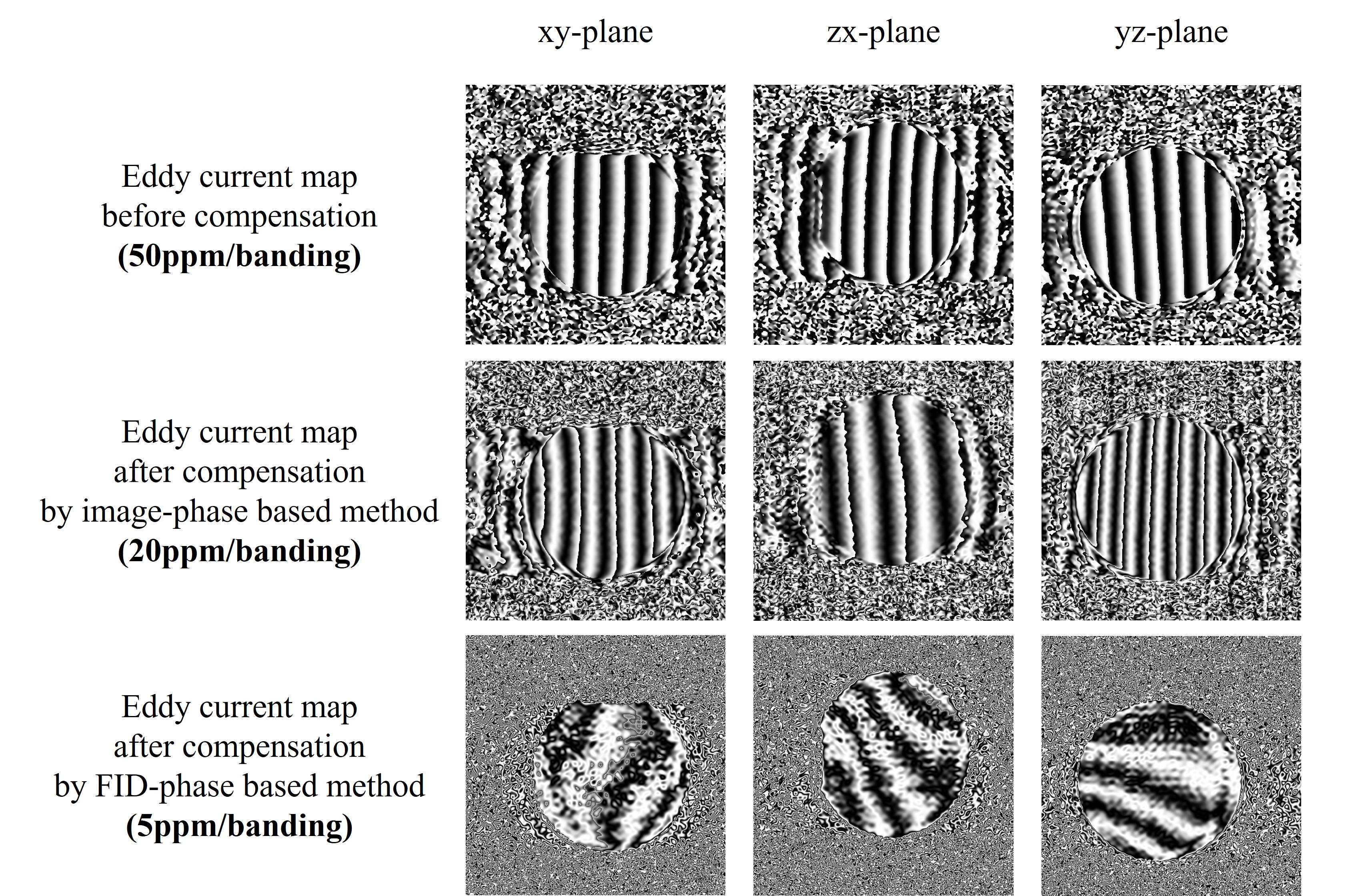
Figure 3 and 4 show the results of all on-axis and cross-term eddy-current-induced gradients we measured by the image-phase based method and FID-phase based method. Both results show that after compensating the gradient system using the information collected from phantoms, the influence of eddy currents was reduced. The fast-decaying cross-term eddy current measured by the large phantom was inaccurate, which may affect the final compensation result.Figure 5 shows maps of eddy current fields (Eddy current maps) before and after compensation. Each 2π variation in phase forms a banding. Then we calculate the equivalent fields shift from the phase and finally get these maps. Number of bandings represents amplitude of residual eddy current. The effects are reduced from 350ppm to about 240ppm and 20ppm by compensation after gaining data from these two measurement techniques.
Conclusions
We used image-phase based and FID-phase based methods to measure the eddy-current-induced gradients in our permanent 64mT low-field MRI system. The first method had simple experimental setup while losing fast-decaying cross-term information. And the second method improved the acquisition efficiency but require additional hardware. Both methods reduced the eddy-current-induced effects.Acknowledgements
Wuxi Marvel Stone Healthcare Research Grant, 23H010102762.References
1. Ahn, C. B., and Z. H. Cho. Analysis of the eddy-current induced artifacts and the temporal compensation in nuclear magnetic resonance imaging. IEEE transactions on medical imaging 10.1 (1991): 47-52.
2. Bhat, Seema S., et al. Low‐field MRI of stroke: challenges and opportunities. Journal of Magnetic Resonance Imaging 54.2 (2021): 372-390.
3. De Zanche, Nicola, et al. NMR probes for measuring magnetic fields and field dynamics in MR systems. Magnetic Resonance in Medicine: An Official Journal of the International Society for Magnetic Resonance in Medicine 60.1 (2008): 176-186.
4. Spees, William M., et al. Quantification and compensation of eddy-current-induced magnetic-field gradients. Journal of magnetic resonance 212.1 (2011): 116-123.
5. Robison, Ryan K., et al. Correction of B0 eddy current effects in spiral MRI. Magnetic resonance in medicine 81.4 (2019): 2501-2513.
6. Morich, Michael A., et al. Exact temporal eddy current compensation in magnetic resonance imaging systems. IEEE transactions on medical imaging 7.3 (1988): 247-254.
7. Terpstra, M., P. M. Andersen, and R. Gruetter. Localized eddy current compensation using quantitative field mapping. Journal of Magnetic Resonance 131.ARTICLE (1998): 139-143.
Figures