4034
Using Amide Proton Transfer Imaging to Detect Alzheimer’s Disease Pathology in Mouse Models1Department of Electrical and Computer Engineering, Whiting School of Engineering, Johns Hopkins University, Baltimore, MD, United States, 2Department of Radiology, School of Medicine, Johns Hopkins University, Baltimore, MD, United States, 3Department of Anesthesiology and Critical Care Medicine, School of Medicine, Johns Hopkins University, Baltimore, MD, United States, 4Department of Biomedical Engineering, Whiting School of Engineering, Johns Hopkins University, Baltimore, MD, United States, 5Department of Mechanical Engineering, Whiting School of Engineering, Johns Hopkins University, Baltimore, MD, United States
Synopsis
Keywords: Alzheimer's Disease, CEST & MT, Alzheimer's Disease
Motivation: APTw imaging can detect abnormal proteins associated with AD, but the APT signal is confounded by the NOE signal, which affects the diagnostic performance.
Goal(s): We want to separate APT and NOE signals and see if the clean signals are better biomarkers for AD diagnosis than APTw signal.
Approach: EMR fitting was performed voxel-wise. Group-based analysis of fitted APT#, NOE# and APTw signal values was performed inside cortex and hippocampus.
Results: APT# and NOE# provide better contrast than APTw for AD diagnosis. The impact of NOE may explain the discrepancy between animal and human studies for AD.
Impact: The fitted APT# and NOE# signals provide better diagnostic values for AD compared to traditional APTw imaging. The impact of NOE may explain the discrepancy between animal and human studies for AD and is worthy of further study.
Introduction
Alzheimer's disease (AD) is the most common type of dementia all over the world. MRI is an important tool for non-invasive diagnosis of AD. Amide proton transfer (APT) imaging,1 a type of chemical exchange saturation transfer (CEST) MRI, may be promising in the diagnosis of AD because it can detect endogenous mobile proteins and peptides, such as soluble Aβ and tau oligomers associated with AD.2 However, due to the use of different AD models and ages, as well as different MRI scanners, pulse sequences and data processing methods, the current results are hard to compare.3-10 In this work, we applied APT imaging to two AD mouse models and used a novel CEST quantification method, called extrapolated semi-solid magnetization transfer reference (EMR),11 to quantify APT and nuclear Overhauser effect (NOE) signals.Method
20 mice, including 5 Tau P301S and 5 wild-type, and 5 APPswe/PSEN1dE9, and 5 wild-type, aged at 2.5 to 3 months, were used in this study. Due to the small sample sizes, the Tau and APP mice were combined as the AD group, while two wild-type mice were combined as the control group. MR imaging was performed on a Bruker 11.7T MRI scanner. APT images with 31 unique offsets were acquired at four different RF saturation powers (0.7, 1.3, 2, and 4μT), and other parameters were: saturation time = 3 sec, FOV = 19.2×19.2 mm2, matrix = 64×64, thickness = 1 mm, 43 offsets = 200(NA=2), 20, 18, … 6, ±4, ±3.75, ±3.5(NA=6), ±3.25, ±3, ±2.5, ±2, … ±0.25, and 0 ppm. Water saturation transfer shift referencing (WASSR) images were acquired for correcting B0 inhomogeneity. T1 map and T2 maps were calculated based on Bruker’s RARE and MSME methods.The conventional APTw image is calculated by MTRasym(3.5ppm) = [Ssat(-3.5ppm) – Ssat(+3.5ppm)] / S0 = Zexp(-3.5ppm) - Zexp(+3.5ppm). The EMR fitting was performed, as proposed previously.11 Then, APT# and NOE# were calculated: APT# = ZEMR(3.5ppm) - Zexp(3.5ppm) and NOE# = ZEMR(-3.5ppm) - Zexp(-3.5ppm). ROIs (cortex and hippocampus) were manually drawn on both sides. The median values of T1, T2, APTw, APT# and NOE# maps in the ROIs were counted for each mouse. Group-based analyzed of these values were performed. Levene’s test was performed to test the equality of variance, and a t-test (for equal variance) or a Welch’s test (for unequal variance) was followed to test the statistical significance.
Results and Discussion
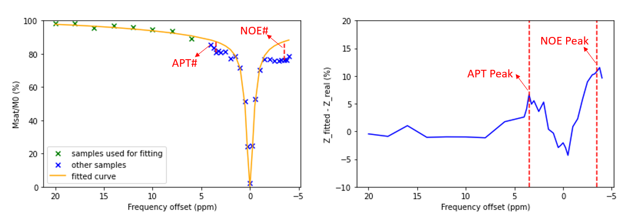
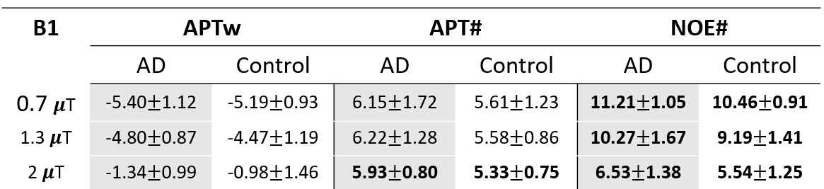
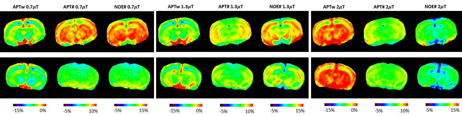
Figure 1 shows an example of EMR fitting for an AD mouse (B1 = 0.7μT). The APT signal was peaked at 3.5ppm downfield from the water. The average APTw, APT# and NOE# signal values for three different B1 powers for AD and control groups were listed in Table 1. For all three powers, higher APT# and NOE# signal intensities were observed in the AD group. APT# in 2μT and NOE# in 0.7, 1.3, 2μT showed significant differences between two groups (p < 0.05). There were no statistically significant differences in APTw signals between AD and control groups in all B1 powers. The T1, T2 values were 2259 ± 186 ms, 39.60±0.70 ms in AD group and 2265±137 ms, 39.83±0.73 ms in control group. No statistically significant difference was found.Based on the definition, APTw = APT# - NOE#. Both APT# and NOE# were higher in AD group, so after subtraction the contrast between AD and control cases were lost to some extent (Figure 2). This suggests that using EMR fitting to separate APT# and NOE# signals can provide better contrast for AD than simply applying APTw imaging. The increase of APT# signal in AD rats was thought to be attributed to the accumulation of abnormal proteins like soluble Ab and tau oligomers, yet the reason of high NOE# signal in AD rats is still to be studied. In most human studies, however, NOE is not a more dominant effect compared to APT so the APTw signal in AD patients is higher than in healthy volunteers7. The mechanism behind this discrepancy between animal and human studies deserves more in-depth researches and experiments.
Conclusion
The EMR fitting method can separate the contribution of APT# and NOE# signals and provide better contrast than APTw imaging for AD studies. Higher APT# and NOE# signals were observed in AD group. The impact of NOE is worthy of further study.Acknowledgements
No acknowledgement found.References
1. Zhou J et al. J Magn Reson Imaging. 2019;50:347–364.
2. Cline EN et al. J Alzheimer's Dis. 2018;64:S567-S610.
3. Wang R et al. Chin Med J. 2015;128:615–9.
4. Wells JA et al. NeuroImage. 2015;111:369-378.
5. Holmes HE et al. Neurobiol Aging. 2016;39:184-194.
6. Chen L et al. NeuroImage. 2019; 188:380-390.
7. Zhang Z et al. NeuroImage. 2020; 25:102-153.
8. Oh JH et al. Korean J Radiol. 2021;22:770-781
9. Huang J et al. Magn Reson Imaging. 2022;87:1529–1545.
10. Li C et al. Magn Reson Letters. 2023;3:22-30.
11. Heo HY et al. Magn Reson Med. 2016;75:137-149.
Figures