3942
EPI Phase Correction revisited - Beat Phenomena and Transient States1Biomedical Magnetic Resonance, Physikalisch-Technische Bundesanstalt (PTB), Braunschweig and Berlin, Germany, 2Institute for Biomedical Engineering, University and ETH Zurich, Zurich, Switzerland, 3Physikalisch-Technische Bundesanstalt (PTB), Braunschweig and Berlin, Germany, 4Department of Medical Engineering, Technische Universität Berlin, Berlin, Germany, 5Einstein Centre Digital Future, Berlin, Germany
Synopsis
Keywords: System Imperfections, System Imperfections: Measurement & Correction, Data Acquisition, Data Processing, Gradients, Image Reconstruction
Motivation: For EPI, beat phenomena can occur and result in a slowly varying, erroneous phase component caused by mechanical resonances of the gradient system. Current phase correction approaches do not account for this error.
Goal(s): Improving EPI correction by characterization of gradient-induced, time-varying errors of zeroth and first spatial order.
Approach: EPI image projections of a spherical phantom were acquired by omitting the phase encoding blips. The resulting x-ky-data enable a characterization of zeroth- and first-order effects separately.
Results: The mechanical properties of the gradient system result in a transient state during which an erroneous, temporally and spatially modulated magnetic field gradient occurs.
Impact: EPI is a widely applied fast imaging technique but sensitive to gradient-induced magnetic field deviations. Therefore, phase correction is of utmost importance and may be improved by the proposed characterization of slowly varying, erroneous phases.
Introduction
Echo-planar imaging1 is inherently sensitive to phase deviations caused by B02, susceptibility3 and trajectory imperfection4. Even-odd echo discrepancies due to B05 and sample shifts6 due to unknown eddy currents and gradient delays result in undesired ghosting and diminished image quality. Numerous correction methods have been proposed, including additional reference scans7, 2D phase higher-order spatial mapping8 and time-dynamic eddy current corrections9. Magnetic field monitoring enables correction for those10,11 at the expense of additional hardware. An imaging based correction for both spatial and temporal dependence of erroneous phases, however, has not been proposed so far. In the current work, insights in the temporal and spatial behavior phase deviations are provided and the existence of a transient phase for oscillating readouts such as EPI is shown and explained theoretically.Theory
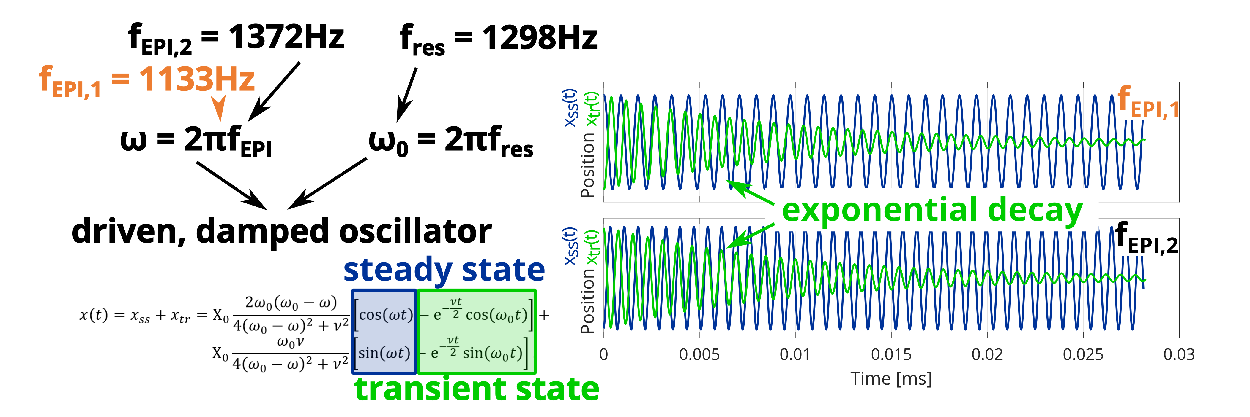
The oscillating behavior of MRI gradient systems (GS) has been investigated in a previous work12. The theoretical description of the GS as a damped harmonic oscillator when assuming very low damping, small positional deviations from its mechanical equilibrium and employing oscillating readouts such as EPI has been studied previously13. Assuming initial conditions of the zero state for the GS and excitation with a harmonic frequency $$$f_{EPI}$$$ near a mechanical resonance frequency $$$f_{res}$$$ (identified as peaks/dips in the gradient transfer function GIRF or GMTF14), the solution for the position yields $$$x(t)=x_{ss}+x_{tr}$$$, where $$$x_{ss}$$$ and $$$x_{tr}$$$ refer to the steady-state solution and the transient solution, respectively (Figure 1). The latter decays exponentially over time on the order of the inverse of the mechanical damping constant. During the transient phase, a beat phenomenon occurs, resulting in the position being amplitude-modulated by the difference frequency $$$|f_{res}-f_{EPI}|$$$ (Figure 2). The position is assumed to be related to the erroneous phase $$$\Delta\varphi(t’) \propto \int_0^{t’}x(t)\mathrm{d}t$$$.The erroneous phase
$$$\varphi(t’)=\varphi_{ES}(t’)+\varphi_{B0}(t’)+\Delta\varphi(t’)$$$
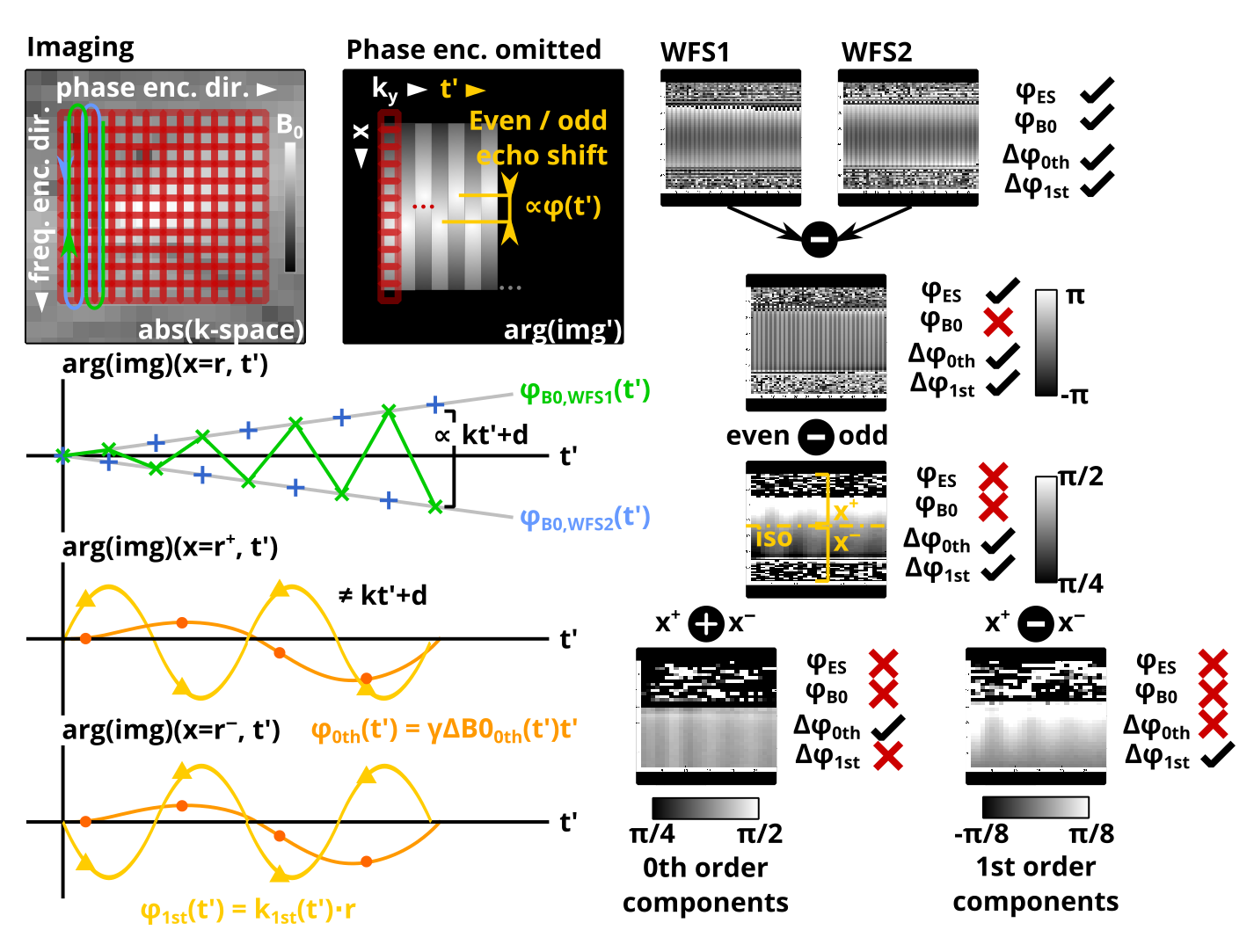
includes phase shifts $$$\varphi_{ES}(t’)$$$ between even and odd echoes, $$$\varphi_{B0}(t’)$$$ due to B0 inhomogeneities and $$$\Delta\varphi(t’)$$$ induced exclusively by the GS. The latter includes erroneous k-space position offset due to 1st order and B0 offsets as a result of 0th order GMTF terms given as $$$\Delta\varphi(t’)=\varphi_{0th}(t’)+\varphi_{1st}(t’)=\gamma\Delta{B0}_{0th}(t’)t'+\Delta\vec{k}_{1st}(t’)\vec{r}$$$ where $$$\Delta{B0}_{0th},\,\Delta \vec{k}_{1st}$$$ and $$$\vec{r}$$$ denote the erroneous terms arising due to 0th and 1st order effects and the spatial position of magnetization, respectively. Assuming a subject or phantom at the isocenter and the isocenter position included in the imaging slice, the components of 0th and 1st order can be distinguished (Figure 3) as they are symmetric and anti-symmetric around the isocenter.
Methods
A 3T MRI system (Philips Healthcare, Best, the Netherlands) and a vendor-supplied EPI sequence was used to acquire a non-oblique slice of a stationary, spherical phantom positioned at the isocenter. Additional measurements, while omitting phase encoding and inverting the sign of the readout gradient, resulted in 1D projections along ky (1DFT) with different water/fat shift directions (WFS1 and WFS2) along the z gradient axis. The frequency of the EPI readout was varied between $$$f_{EPI}=[1298, 1448]\mathrm{Hz}$$$ with TE=const. while the mechanical resonance frequency of the corresponding gradient axis was identified earlier as $$$f_{res}=1298\mathrm{Hz}$$$. Data reconstruction was performed with MRecon (GyroTools LLC, Winterthur, Switzerland) without EPI phase correction and inverse Fourier transform in ky direction; the 1DFT data processing steps are shown in Figure 3.Results & Discussion
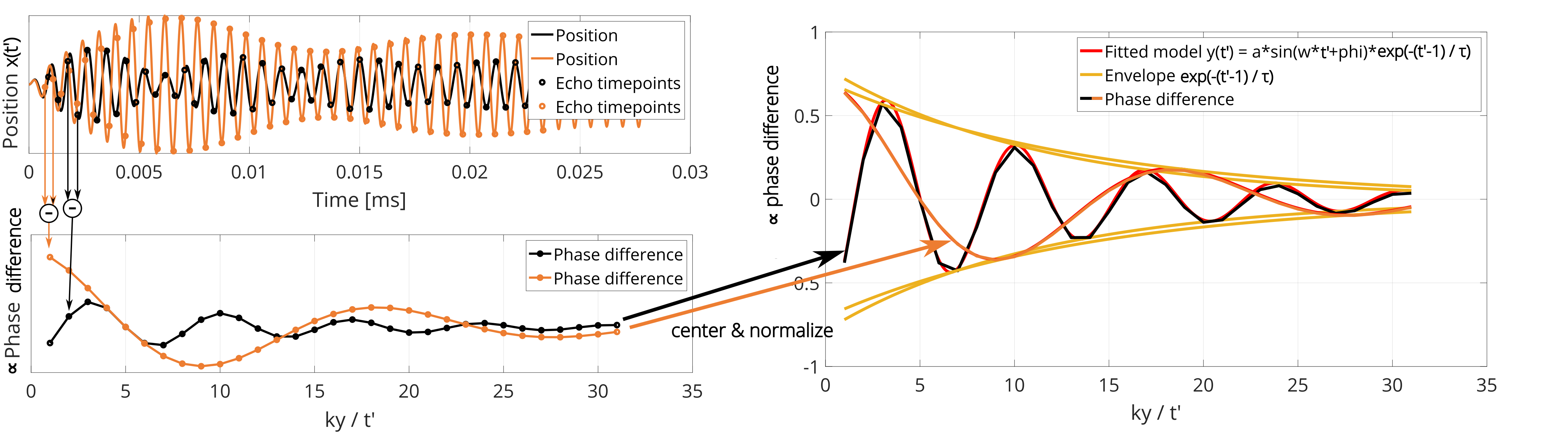
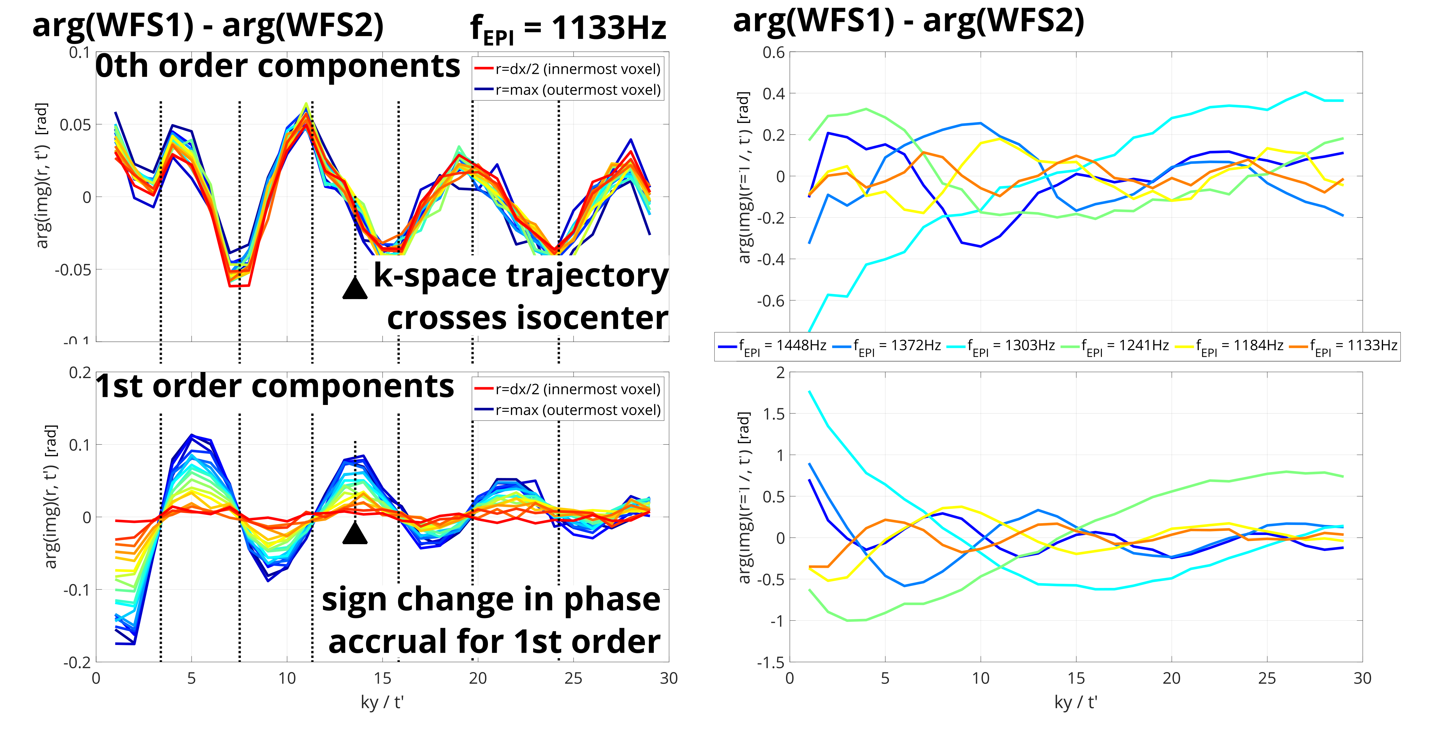
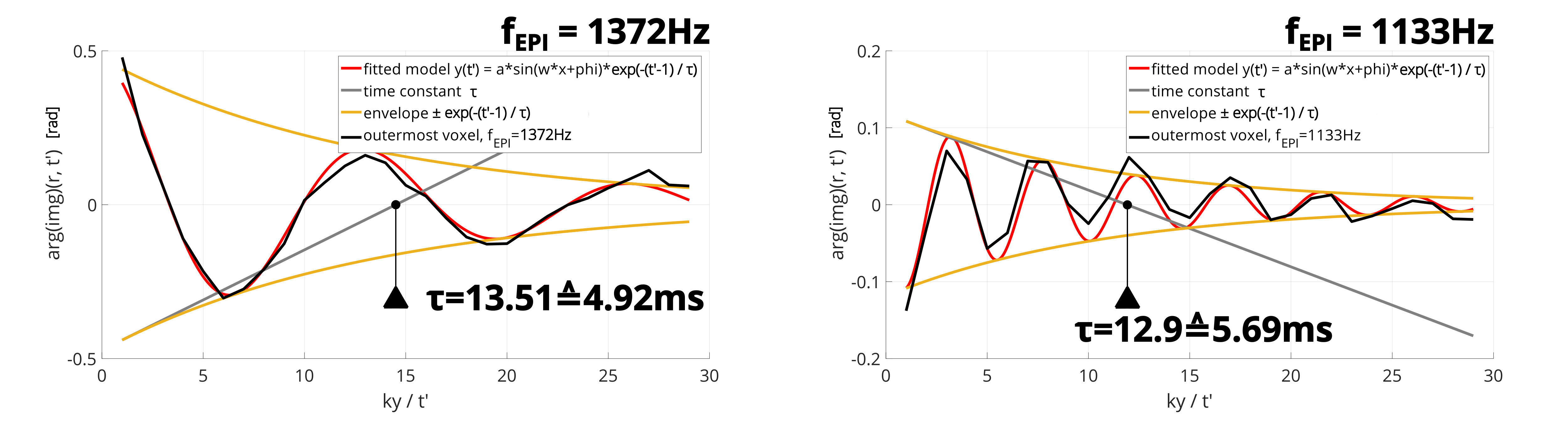
In Figure 4, left, phase plots from experimental data for varying distances from the isocenter for 0th and 1st order are shown; the mean of the plots has been subtracted for better interpretability. Against intuition, the 0th order component is not increasing throughout since the exponential decay of the transient solution counteracts its linear amplitude growth in time, causing it to start decreasing at $$$t’=\tau$$$ (cf. Figure 5). As expected, 1st order components are spatially dependent and their phase over time follows the exponential decay. In Figure 4, right, the amplitude of the observed beat is dependent on the frequency $$$f_{beat} = |f_{EPI}-f_{res}|$$$. A maximum of 2rad was found for $$$f_{EPI}=1303\mathrm{Hz}$$$. In comparison, a minimum main field inhomogeneity of 0.1ppm recommended for EPI15 would lead to 2.5rad for a comparable acquisition time.Figure 5 presents exemplary fitting results for measurement data using a sinusoidal model with exponential decay. The time constant $$$\tau$$$ can be identified which is related to the mechanical damping constant $$$\nu$$$. The robust fitting procedure was performed at several $$$f_{EPI}$$$ and spatial positions (not shown here).
Conclusion
We have presented a manifestation of the beat phenomenon in oscillating readouts causing both spatially dependent and independent erroneous phases varying in a non-linear fashion over the readout duration. Current EPI phase correction approaches assume spatial invariance and linear behavior in time and could be improved by incorporation of the beat phenomenon.Acknowledgements
The authors acknowledge funding of the Platform for Advanced Scientific Computing of the Council of Federal Institutes of Technology (ETH Board), Switzerland. The authors would like to thank Karl Treiber for the possibility to scan at UZH.References
1. Mansfield P. Multi-planar image formation using NMR spin echoes. J Phys C Solid State Phys. 1977;10(3):55-58. doi:10.1088/0022-3719/10/3/004
2. Jezzard P, Balaban RS. Correction for geometric distortion in echo planar images from B0 field variations. Magn Reson Med. 1995;34(1):65-73. doi:10.1002/mrm.1910340111
3. DeLaPaz RL. Echo-planar imaging. Radiographics. 1994;14(5):1045-1058. doi:10.1148/radiographics.14.5.7991813
4. Vannesjo SJ, Graedel NN, Kasper L, et al. Image reconstruction using a gradient impulse response model for trajectory prediction. Magn Reson Med. 2016;76(1):45-58. doi:10.1002/mrm.25841
5. Buonocore MH, Gao L. Ghost artifact reduction for echo planar imaging using image phase correction. Magn Reson Med [Internet]. 1997 Jul;38(1):89–100. Available from: https://onlinelibrary.wiley.com/doi/10.1002/mrm.1910380114
6. Reeder SB, Atalar E, Bolster BD, McVeigh ER. Quantification and reduction of ghosting artifacts in interleaved echo- planar imaging. Magn Reson Med. 1997;38(3):429–39.
7. Hu X, Le TH. Artifact reduction in EPI with phase-encoded reference scan. Magn Reson Med. 1996;36(1):166–71.
8. Chen NK, Wyrwicz AM. Removal of EPI Nyquist ghost artifacts with two-dimensional phase correction. Magn Reson Med. 2004;51(6):1247–53.
9. Jezzard P, Barnett AS, Pierpaoli C. Characterization of and correction for eddy current artifacts in echo planar diffusion imaging. Magn Reson Med. 1998;39(5):801–12.
10. Barmet C, De Zanche N, Pruessmann KP. Spatiotemporal magnetic field monitoring for MR. Magn Reson Med. 2008;60(1):187–97.
11. Wilm BJ, Barmet C, Pavan M, Pruessmann KP. Higher order reconstruction for MRI in the presence of spatiotemporal field perturbations. Magn Reson Med. 2011;65(6):1690–701.
12. Dillinger H, Kozerke S, Guenthner C. Direct Comparison of Gradient Modulation Transfer Functions and Acoustic Noise Spectra of the same MRI at High- (3T) and Lower-Field (0.75T). Proc. Intl. Soc. Mag. Reson. Med. 30 (2021)
13. Dillinger H, Kozerke S. Beat Phenomena in MRI - Theoretical and Experimental Description of the Impact of Mechanical Resonances on Fast Readouts. In: Joint Annual Meeting ISMRM-ESMRMB ISMRT 31st Annual Meeting. 2022.
14. Vannesjo SJ, Haeberlin M, Kasper L, Pavan M, Wilm BJ, Barmet C, et al. Gradient system characterization by impulse response measurements with a dynamic field camera. Magn Reson Med. 2013;69(2):583–93.
15. Jackson E, Bronskill M, Drost D, Och J, Pooley R, Sobol W, et al. AAPM n°100 - Acceptance Testing and Quality Assurance Procedures for Magnetic Resonance Imaging Facilities. AAPM report No. 100. 2010. 1–32 p.
Figures