3934
FESTiVE - implicit Field Estimator for Spatio-Temporally Varying Eddy Currents1Electrical Engineering, Stanford University, Stanford, CA, United States, 2Radiology, Stanford University, Stanford, CA, United States
Synopsis
Keywords: System Imperfections, Gradients
Motivation: Gradient imperfections from eddy currents and trajectory error cause image artifacts. NMR field probes can accurately measure these imperfections to achieve high-quality imaging, but require additional hardware and cost.
Goal(s): Develop an alternative imaging-based approach to estimate gradient imperfections by leverage the encoding capability of modern multi-channel receivers and neural networks for implicit Fourier phase representation.
Approach: Simulated spiral imaging acquisition with eddy current and low-gradient sequences without eddy effects. Trained MLPs to convolutionally represent gradient phase imperfections in k-space as a function of time.
Results: MLP estimates spatio-temporal phase to high accuracy, showing promise for high-order phase estimation without NMR field probes.
Impact: We propose an algorithmic imaging-based alternative approach to field probe for gradient characterization. This enables enhanced image reconstruction for high-slew MRI without external hardware, potentially revolutionizing fast acquisition MRI techniques and broadening their application.
Introduction
Spiral and echo-planar imaging have grown in popularity due to their ability to more fully utilize the limits of the gradient systems for fast acquisition. However, the necessarily high slew rates introduce gradient imperfections, such as eddy currents and trajectory errors1,2. Typically, mitigation involves calibration scans for gradient characterization and phase modeling to adjust distortions during reconstruction. One-dimensional gradient corrections has been shown using self-encoded slice selection algorithms, negating extra hardware needs3,4. Extending phase characterization with NMR field probes enhances reconstruction but adds cost and complexity, and is restricted to 3rd-order spherical harmonics1,5.Techniques that rely on learned correlations in k-space from multichannel receiver training data have been successful in performing k-space interpolation (GRAPPA6, SPIRIT7) and cartesian gridding for faster reconstruction (GROG8). Recently, multi-layer perceptrons (MLP) have been proposed to implicitly represent multi-channel k-space relationships, improving speed and performance for GROG9. Our contribution extends this idea, exploiting k-space correlations in characterizing gradient imperfections though a data-driven approach: implicit Field Estimators for Spatio-Temporally Varying Eddy currents (FESTiVE). This can be performed from a calibration scan without external hardware, relying only on parallel receive coils as probes for gradient characterization, providing additional flexibility to estimate higher-order terms beyond third-order limitations.
Background and Theory
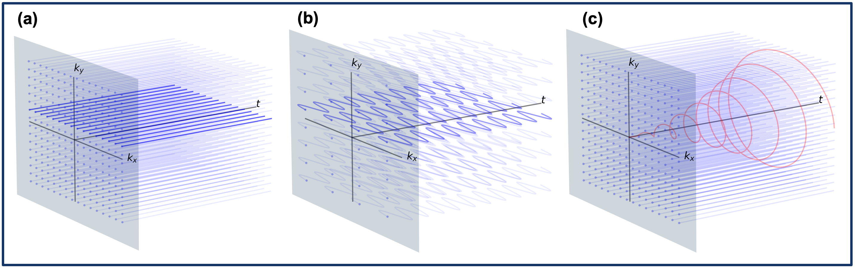
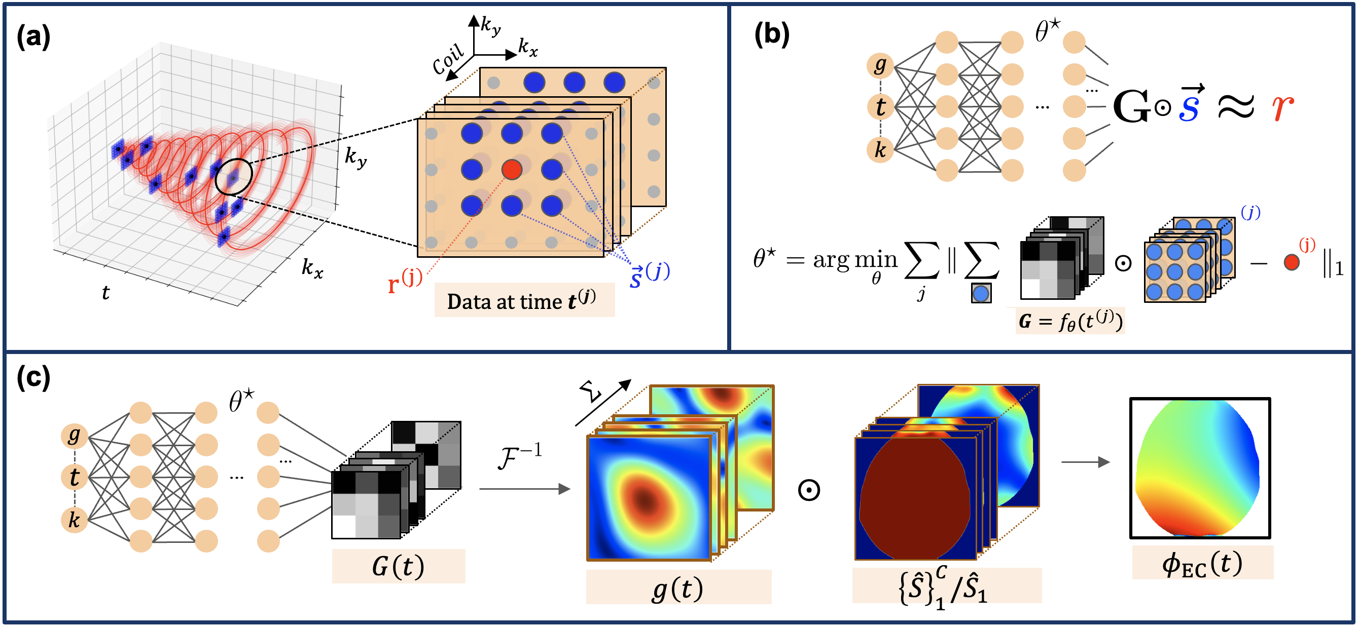
We typically design a gradient waveform to produce a trajectory $$$k(t)$$$ to sample k-space efficiently. Define signal from the $$$c$$$th coil with sensitivity $$$S_c(r)$$$ as:$$s_c(t)=\int_{r}S_{c}(r)m(r)e^{j2{\pi}{k(t)^T}r}dr$$We model eddy current effects in the signal equation with an additional phase term: $$\tilde{s}_c(t)=\int_{r}S_{c}(r)m(r)e^{j2{\pi}{k(t)^T}r}e^{j \phi_c(r,t)}dr$$$$$\phi_c(r,t)$$$ is generally smooth both spatially and temporally, as eddy currents induced by gradient switching decay exponentially with time. We propose an approximation to the eddy current phase using a sum of weighted Fourier harmonics:$$e^{j\phi_c(r,t)}=\sum_{k=1}^K\sum_{c=1}^CS_c(r)w_{k,c}(t)e^{j2{\pi}k_k^Tr}$$Weighting these terms over the parallel receive system, we can relate $$$\tilde{s}_c(t)$$$ to eddy current-free k-space. Assuming sensitivity maps in their SVD basis, we project the received signal onto the first basis coil $$$\hat S_1$$$, which is relatively flat in both magnitude and phase:$$\begin{aligned}\tilde{s}_1(t)=&\int_r\hat{S}_1(r)m(r)e^{j2{\pi}k(t)^Tr}\sum_{k=1}^K\sum_{c=1}^C\hat{S}_c(r)w_{k,c}(t)e^{j2{\pi}k_k^Tr}dr\\&=\sum_{k=1}^K\sum_{c=1}^Cw_{k,c}(t)\int_r\hat{S}_1(r)\hat{S}_c(r)m(r)e^{j2{\pi}(k(t)+k_k)^Tr}dr\\&=\sum_{k=1}^K\sum_{c=1}^C\hat{w}_{k,c}(t)s^k_{c}(t)\end{aligned}$$Here, each $$$s^{k}_c(t)$$$ term is an eddy current-free signal offset from $$$\tilde{s}_c(t)$$$ by the spatial frequency $$$k$$$, and $$$\hat{w}_{k,c}$$$ are the Fourier weights relative to $$$\hat S_1(r)$$$. Writing this system compactly as $$$r(t)=G(t)\odot\vec{s}(t)$$$ for $$$r(t)=\tilde{s}_1(t)$$$ as our “target” data along the nominal high-gradient trajectory, and $$$\vec{s}(t)$$$ as the collection of clean data, which we denote the “source” points, the spatio-temporal phase along some nominal trajectory can be represented as a weighted combination of unaffected k-space samples surrounding the original data. $$$\vec{s}(t)$$$ can be collected using sequences designed to cover k-t space with low slew rates as described in $$$\textbf{Figure}{\,}1$$$. Spatial and temporal smoothness of field variations implies that the $$$G(t)$$$ kernels should reside in a low-dimensional space. Thus, we parameterize the set of kernels $$$G(t)$$$ as learnable weights by a neural network $$$f_\theta(t)$$$. Signal data collected along $$$k(t)$$$ and interpolated from the surrounding source space becomes a set of training points for MLP training as shown in $$$\textbf{Figure}{\,}3(b)$$$. The eddy current phase can then be backed out directly from the kernels learned by the network, as in $$$\textbf{Figure}{\,}3(c)$$$.
Methods
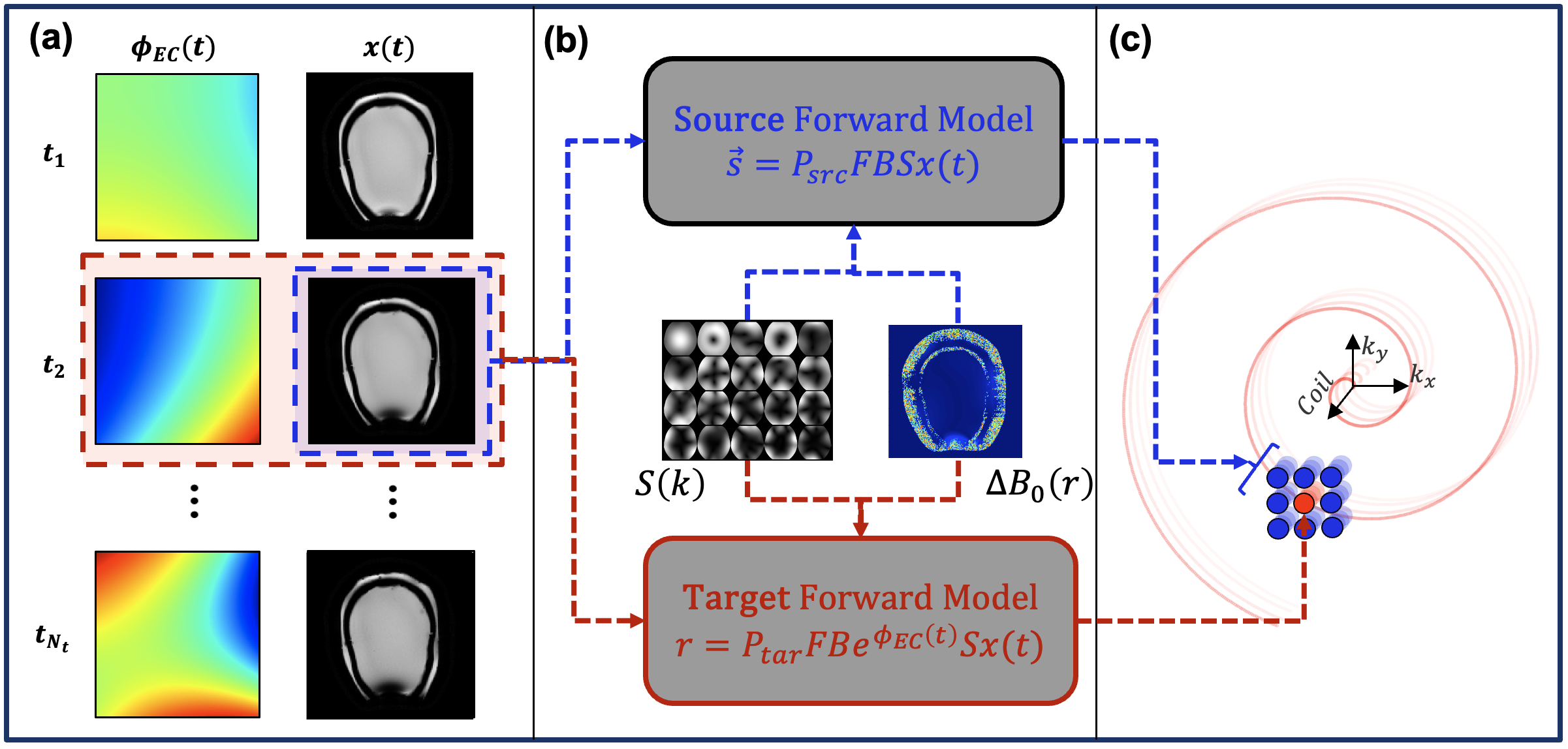
We demonstrate the feasibility of an MLP to estimate gradient inhomogeneities with a simulation of the data acquisition process described in $$$\textbf{Figure}{\,}2$$$. For this, we imaged a phantom ($$$\textbf{Figure}{\,}3(a)$$$) on a 32-channel 3T scanner, with coil sensitivity maps estimated with ESPIRIT10. We acquired a single-shot R=2 variable-density 2D spiral, and measured the gradient imperfections up to third order spherical harmonics using Skope NMR field probes5. We then simulated signal acquisition, applying the Skope-measured fields as trajectory-induced gradient inhomogeneities, to generate source data $$$r(t)$$$, simultaneously collecting the ground truth source points $$$\vec{s}(t)$$$. Signal data was simulated per-timepoint to mimic the time-evolving effects of $$$T_{2}^{\star}(r)$$$, $$$\Delta B_0(r)$$$, and the phase due to $$$\phi_c(r,t)$$$. A 3-layer MLP then estimated the fields by mapping the spiral gradient waveform and time to a Fourier kernel representing the current phase. Training over 100 epochs with an Adam11 optimizer against an $$${\ell}_1$$$-loss on phase mapping error ($$$\textbf{Figure}{\,}3(b)$$$) takes less than 30 seconds on a GPU. The estimated fields are then taken to be the coil-weighted Fourier-transformed kernels ($$$\textbf{Figure}{\,}3(c)$$$).Results and Discussion
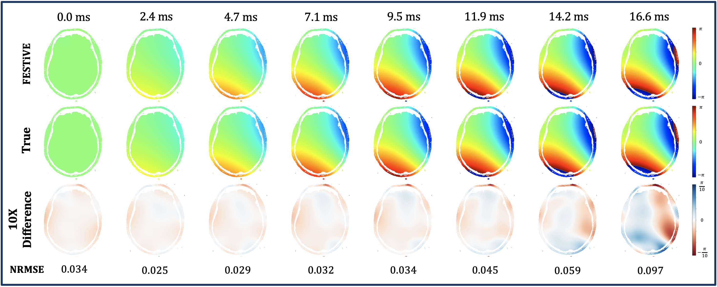
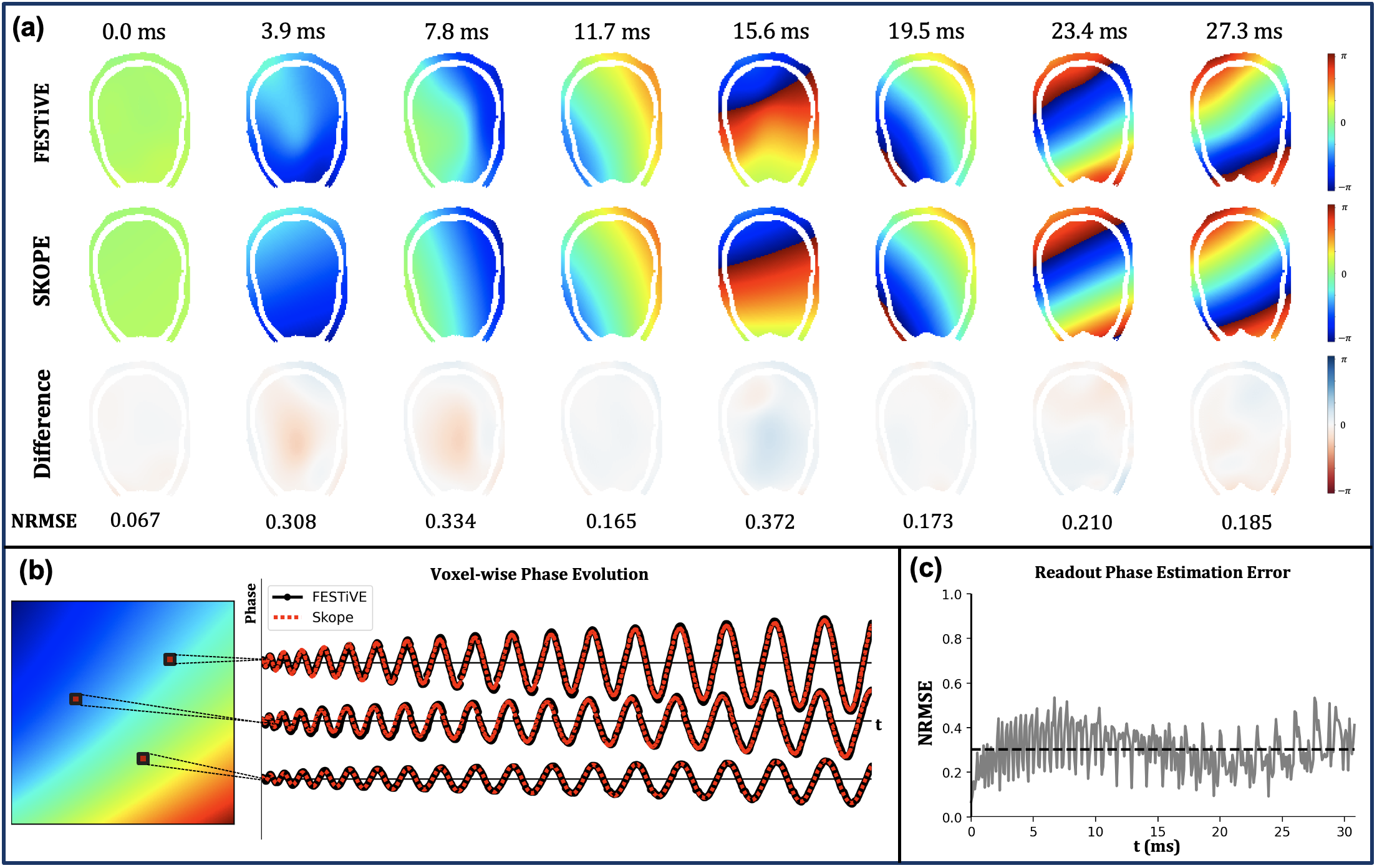
$$$\textbf{Figure}{\,}4$$$ summarizes the results on a toy example, with gradient imperfections modeled as time-decaying spherical harmonics. $$$\textbf{Figure}{\,}5$$$ demonstrates performance on simulated data with eddy currents acquired by Skope probes. $$$\textbf{Figure}{\,}5(b)$$$ shows that the gradient imperfection phase estimated by the MLP closely matches the periodicity and temporal evolution of probe measurements.This work introduces the MLP's capability to discern higher-order Fourier phases. Future research will apply this method to in-vivo gradient characterization. Given the MLP's ability to estimate beyond third-order effects, it may enhance image reconstruction significantly.
Acknowledgements
This work was supported by the National Institutes of Health under grants R01MH116173, R01EB019437, U01EB025162, P41EB030006, R01EB033206, and U24NS129893.References
- Chan, R. W., Von Deuster, C., Giese, D., Stoeck, C. T., Harmer, J., Aitken, A. P., ... & Kozerke, S. (2014). Characterization and correction of eddy-current artifacts in unipolar and bipolar diffusion sequences using magnetic field monitoring. Journal of Magnetic Resonance, 244, 74-84. Elsevier.
- Jezzard, P., Barnett, A. S., & Pierpaoli, C. (1998). Characterization of and correction for eddy current artifacts in echo planar diffusion imaging. Magnetic Resonance in Medicine, 39(5), 801-812. Wiley Online Library.
- Cheng, J. Y. (2007). Gradient Characterization in Magnetic Resonance Imaging (Master of Engineering in Electrical Engineering and Computer Science). Massachusetts Institute of Technology, Cambridge, MA.
- Duyn, J. H., Yang, Y., Frank, J. A., & van der Veen, J. W. (1998). Simple correction method for k-space trajectory deviations in MRI. Journal of Magnetic Resonance, 132(1), 150-153. Academic Press.
- De Zanche, N., Barmet, C., Nordmeyer-Massner, J. A., & Pruessmann, K. P. (2008). NMR probes for measuring magnetic fields and field dynamics in MR systems. Magnetic Resonance in Medicine, 60(1), 176-186. Wiley Online Library.
- Griswold, M. A., Jakob, P. M., Heidemann, R. M., Nittka, M., Jellus, V., Wang, J., ... & Haase, A. (2002). Generalized autocalibrating partially parallel acquisitions (GRAPPA). Magnetic Resonance in Medicine, 47(6), 1202-1210. Wiley Online Library.
- Lustig, M., & Pauly, J. M. (2010). SPIRiT: iterative self-consistent parallel imaging reconstruction from arbitrary k-space. Magnetic Resonance in Medicine, 64(2), 457-471. Wiley Online Library.
- Seiberlich, N., Breuer, F. A., Blaimer, M., Barkauskas, K., Jakob, P. M., & Griswold, M. A. (2007). Non-Cartesian data reconstruction using GRAPPA operator gridding (GROG). Magnetic Resonance in Medicine, 58(6), 1257-1265. Wiley Online Library.
- Abraham, D., Nishimura, M., Cao, X., Liao, C., & Setsompop, K. (2023). Rapid Non-cartesian Reconstruction Using an Implicit Representation of GROG Kernels. arXiv preprint arXiv:2310.10823.
- Uecker, M., Lai, P., Murphy, M. J., Virtue, P., Elad, M., Pauly, J. M., ... & Lustig, M. (2014). ESPIRiT—an eigenvalue approach to autocalibrating parallel MRI: where SENSE meets GRAPPA. Magnetic Resonance in Medicine, 71(3), 990-1001. Wiley Online Library.
- Kingma, D. P., & Ba, J. (2014). Adam: A method for stochastic optimization. arXiv preprint arXiv:1412.6980.
Figures