3931
How to reduce trajectory errors caused by non-linear gradient amplifier characteristics1Department of Diagnostic and Interventional Radiology, University Hospital Würzburg, Würzburg, Germany, 2Ostbayerische Technische Hochschule Amberg-Weiden, Amberg/ Weiden, Germany, 3Advanced Clinical Imaging Technology (ACIT), Siemens Healthineers International AG, Zurich, Switzerland, 4Swiss Center for Musculoskeletal Imaging (SCMI), Balgrist Campus, Zurich, Switzerland, 5Advanced Clinical Imaging Technology (ACIT), Siemens Healthineers International AG, Lausanne, Switzerland, 6Siemens Healthcare GmbH, Erlangen, Germany
Synopsis
Keywords: System Imperfections, System Imperfections: Measurement & Correction, Linear Time-invariant Model
Motivation: The gradient system transfer function (GSTF) can correct k-space distortions arising from gradient imperfections, but is limited by assuming a linear, time-invariant gradient system.
Goal(s): We wanted to investigate the linearity of the gradient signal path before and after the gradient power amplifier.
Approach: We compared transfer functions for different segments of the gradient chain, measured with positive and negative test pulses. We then predicted the waveform of a trapezoidal gradient with the transfer functions, and quantified the error of the predicted k-space.
Results: Using a transfer function based on the gradient amplifier currents halved the errors on the predicted k-space coordinates.
Impact: The current-based transfer function could enable a fully automated k-space trajectory determination with doubled accuracy compared to the gradient system transfer function, without special hardware or lengthening scan times. This could help with the clinical translation of non-Cartesian MRI acquisitions.
Introduction
Non-Cartesian k-space trajectories are prone to artifacts arising from gradient imperfections, often hindering their clinical usability. A broadly used tool to mitigate gradient imperfections is the gradient system transfer function (GSTF), which characterizes the gradient system’s transmission behavior assuming linearity and time-invariance (LTI)1. However, these assumptions are undermined by non-linear characteristics of the gradient power amplifiers (GPA)2, or heating of the gradient coils3,4. We previously demonstrated that these LTI-violations can cause errors in the predicted gradient waveforms5,6. Here, we examined the linearity of the whole gradient signal chain, as well as the signal paths from the sequence to the GPA, and from the GPA to the gradient field, separately. We wanted to quantitatively assess the influence of nonlinearities in the amplifier on the GSTF and the resulting trajectory predictions.Methods
We measured three transfer functions: 1) A sequence-to-field-transfer function (TF), i.e. the GSTF, using the prescribed gradient waveform as input, and the measured field evolution as output. 2) A sequence-to-current-TF, using the output current of the GPA as output. 3) A current-to-field-TF, using the GPA’s output current as input, and the measured field as output. The field measurements followed the thin slice method7. For the current measurements, the ADC of our research application sequence picked up the signal from a built-in sensor in the GPA proportional to the output current. We used 10 triangular gradient pulses for the TF measurements, and measured each TF once with positive and once with negative triangle amplitudes. We then used a trapezoidal gradient8 to quantify the prediction errors of the different TFs. The experiments were conducted on a 3T scanner (MAGNETOM Prismafit, Siemens Healthcare, Erlangen, Germany), with the head coil and a spherical phantom. Table 1 contains all the measurement details.Results
Figure 1 shows the six TFs for the physical z-axis of our gradient system, and the magnitude difference between the TFs measured with positive and negative triangles. For the sequence-to-field-TF and the sequence-to-current-TF, we see distinct deviations between the functions with positive and negative input and output (Fig. 1G, H). In contrast, the difference is just noise for the current-to-field-TFs (Fig. 1I). Figure 2 shows the measured and calculated waveforms of the positive trapezoidal gradient, and the differences between measurements and calculations. The calculation was done with the TF of the positive triangles and with the TF of the negative triangles of the respective signal path. In all cases, small differences between measurement and prediction at the start and end of the edges of the trapezoid were observed. Only for the current-to-field-segment, both TFs produce almost identical waveform predictions (Fig. 2F). In Figure 3, we examine the k-space coordinates of the trapezoid. On the left, we compare the measurement to the prediction with the sequence-to-field-TF, and on the right to the prediction with the current-to-field-TF. We clearly see that the sequence-to-field-TF produces larger deviations, which is also reflected in the root-mean-squared-error (0.17 vs. 0.08).Discussion
The deviations between the “positive” and “negative” TFs for the sequence-to-field-signal and the sequence-to-current-signal indicate that the signal path up to the GPA output violates the linearity assumption. When looking at the predictions for the trapezoid, we can actually see that none of the examined signal paths perfectly fulfills the LTI assumption, because there are always small deviations from the measurement. However, the deviations are smallest for the predictions by the current-to-field-TFs. This is also the only model that is independent of the sign of the triangular pulses used for its determination, which points to a better LTI compliance than the sequence-to-field- or sequence-to-current-model possess. Relevant for imaging applications is, of course, the accuracy of the associated k-space coordinates. Larger errors of the gradient prediction may be irrelevant if they are cancelled out by integration. However, this is not the case for the sequence-to-field-model (c.f. Figure 3). The current-to-field-model produces smaller absolute k-space-errors throughout the considered time window, resulting in about half the RMSE. These results quantitatively confirm the qualitative observations made earlier by Rahmer et al. on a Philips scanner2, who showed that a trajectory correction with a current-based GSTF yields better image quality than the traditional GSTF.Conclusion
We showed that an LTI model of the gradient system that uses the GPA current as input adheres better to the LTI assumptions and leads to smaller errors in the trajectory prediction that the traditional GSTF model. If the GPA current could be monitored concurrently, this would offer the possibility for improved fully automated k-space trajectory corrections without needing special hardware, such as a field monitoring camera9.Acknowledgements
No acknowledgement found.References
1. Vannesjo SJ, Graedel NN, Kasper L, et al. Image reconstruction using a gradient impulse response model for trajectory prediction. Magn Reson Med. 2016;76(1):45-58. doi:10.1002/mrm.25841
2. Rahmer J, Schmale I, Mazurkewitz P, Lips O, Börnert P. Non‐Cartesian k‐space trajectory calculation based on concurrent reading of the gradient amplifiers’ output currents. Magn Reson Med. 2021;85(6):3060-3070. doi:10.1002/mrm.28725
3. Stich M, Pfaff C, Wech T, et al. The temperature dependence of gradient system response characteristics. Magn Reson Med. 2020;83(4):1519-1527. doi:10.1002/mrm.28013
4. Nussbaum J, Dietrich BE, Wilm BJ, Pruessmann KP. Thermal variation in gradient response: measurement and modeling. Magn Reson Med. 2022;87(5):2224-2238. doi:10.1002/mrm.29123
5. Scholten H, Köstler H. Towards gradient perturbation correction in diffusion weighted imaging based on the gradient system transfer function. In: Proceedings of the 2022 Joint Annual Meeting ISMRM-ESMRMB. ; 2022.
6. Sommer S, Köstler H, Scholten H. Modelling the gradient system as linear and time-invariant: Do the assumptions break down at higher field strength? In: Proceedings of the 2023 ISMRM Annual Meeting. ; 2023.
7. Duyn JH, Yang Y, Frank JA, van der Veen JW. Simple Correction Method fork-Space Trajectory Deviations in MRI. J Magn Reson. 1998;132(1):150-153. doi:10.1006/jmre.1998.1396
8. Scholten H, Lohr D, Wech T, Köstler H. Measuring gradient waveforms effectively with fully compensated variable-prephasing. In: Proceedings of the 2023 ISMRM Annual Meeting. ; 2023.
9. Dietrich BE, Brunner DO, Wilm BJ, et al. A field camera for MR sequence monitoring and system analysis. Magn Reson Med. 2016;75(4):1831-1840. doi:10.1002/mrm.25770
Figures
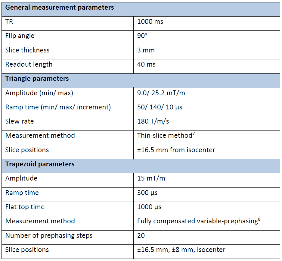
Table 1. Measurement parameters.
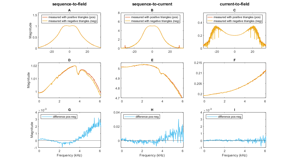
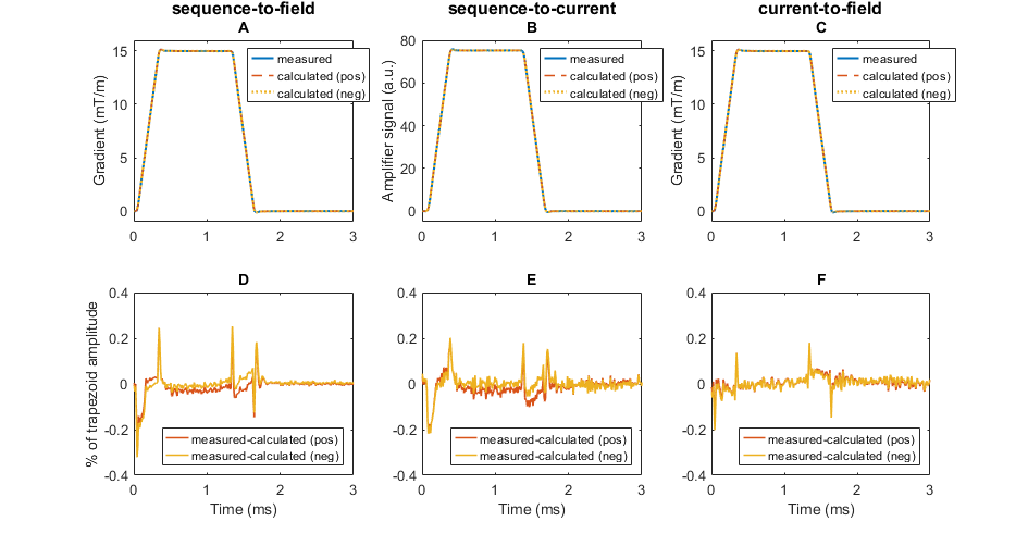
Figure 2. Measured and calculated waveforms of a trapezoidal gradient for the different segments of the gradient signal chain, as in Figure 1. The first row shows the measured trapezoid, and the calculated ones using the transfer functions measured with positive (pos) and negative (neg) triangular pulses. The second row shows the differences between the measured and the two calculated curves.
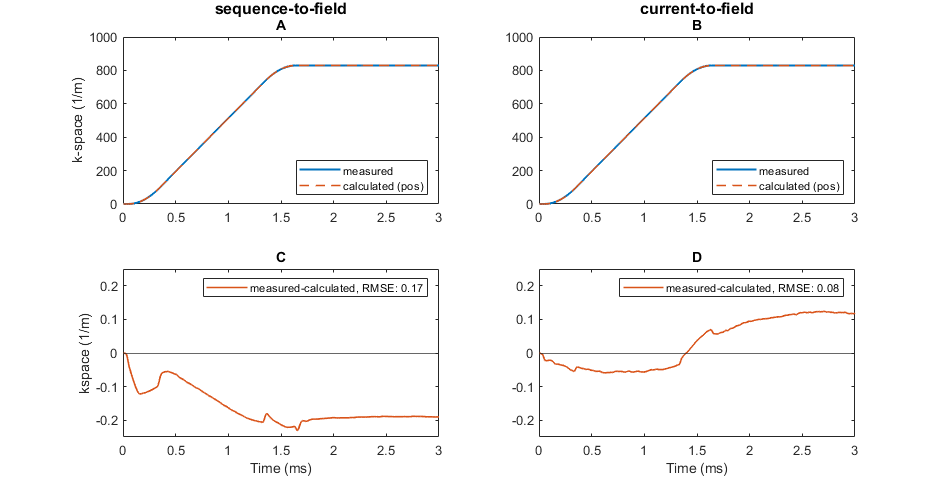
Figure 3. First row: Measured and predicted k-space coordinate of the trapezoidal gradient. Left: Calculation with the GSTF (measured with positive triangles), describing the whole gradient chain. Right: Calculation with the transfer function describing the path from the amplifier current to the generated field (also measured with positive triangles). Second row: Difference between measurement and calculation. The RMSE for the displayed time window (0 to 3 ms) is indicated in the legend.