3913

Calculation of Eddy Power Losses Within the Cryostat Generated by Array or Conventional Gradient Assembly for Arbitrary Pulse Sequences

Manouchehr Takrimi¹ and Ergin Atalar^1,2
¹UMRAM, Bilkent University, Ankara, Turkey, ²Electrical & Electronics Engineering Department, Bilkent University, Ankara, Turkey

Synopsis

Keywords: Gradients, Gradients, Eddy current, Electromagnetic Simulations

Motivation: Existing eddy current calculation methods aren't suitable for fast eddy power loss calculations.

Goal(s): We propose a quick calculation to estimate the time-average eddy power loss within the cryostat, generated by gradient assembly (array or conventional) and arbitrary pulse sequences.

Approach: The frequency response of the fields generated by the gradient assembly elements (array or conventional) on the cryostat's surface is combined with the harmonic components of the driving pulse sequences.

Results: A typical pulse sequence feeds a whole-body conventional x-gradient coil, and the proposed method estimates the time-average dissipated power on the fly, comparable with simulation results reported by commercial software.

Impact: Our method optimizes gradient assembly (array/conventional) tuning, empowering MRI engineers with fast and precise dissipated power estimates. This approach sparks novel research paths, enhancing MRI system efficiency and enabling tailored pulse sequences for gradient coils, advancing the field significantly.

Introduction

Calculating cryostat heating caused by complicated induced eddy currents is difficult. Although different numerical methods have been deployed to calculate the eddy currents, such as the finite difference time domain (FDTD) method^1-3, the finite element method (FEM)⁴, and the Multi-layer integral method (MIM)^5-7, almost all of them are computationally extensive for real-time estimations. Using the Poynting theorem, we propose a systematic approach⁸ to estimate and control the time-average eddy power loss within the cryostat body for arbitrary coil assembly and pulse sequences. It is a fast and accurate solution to estimate the power dissipation in the cryostat region.

Methods

The phasor integral form of the Poynting theorem⁹ for a simple conductive medium of volume $$$V$$$ enclosed by surface(s) $$$S$$$, with no impressed sources inside, reads:$$\int_{V}\frac{1}{2}{\left(\overline{E}\cdot\overline{J}^{\,*}\right)dv+j4\pi{f}\left[\int_{V}\frac{1}{4}{\left(\overline{B}\cdot\overline{H}^{\,*}\right)\!dv}-\!\int_{V}\frac{1}{4}{\left(\overline{E}\cdot\overline{D}^{\,*}\right)\!dv}\right]}=-\oint_{S}\frac{1}{2}{\left(\overline{E}\!\times\!\overline{H}^{\,*}\right)\!\cdot\hat{a}_n{ds}},\qquad[1]$$
where $$$\hat{a}_n$$$ is the outward normal unit vector on the closed surface(s) $$$S$$$, $$$\overline{J}$$$ is the volume eddy current density, and $$$f$$$ is the excitation frequency. The first term represents the time-average conversion of the coils’ EM energy into thermal energy (ignoring the vibration). The second and third terms account for the time-average stored magnetic and electric energies within $$$V$$$. Assuming ε, μ, and σ as real constants for the stainless steel cryostat, all integrals are real, and $$$P_{Loss}(f)\!=\!\text{Re}\!\left\{\!-\!\oint_{S}\!\frac{1}{2}{\left(\overline{E}\!\times\!\overline{H}^{*}\!\right)\!\cdot\!{\hat{a}_n}ds }\right\}$$$ represents the total time-average ohmic power loss caused by induced eddy currents. Note that $$$\overline{E}$$$ and $$$\overline{H}$$$ represent the net EM fields and include all nonlinear effects like skin and proximity effects. The fields produced by the coil assembly elements on the cryostat’s surface are simulated and captured for unity amplitude excitation and a set of frequencies with an appropriate spatial resolution. Once the surface EM fields for each coil element are recorded, the total net EM fields can be found by superposition, facilitating the computation of Equation [1]. This approach may require several hours of simulations, depending on the accuracy and the mesh size, but it has only to be computed once for each gradient coil.
Given a gradient pulse sequence of period $$$T$$$, say $$$g(t)$$$, the grand total time-average eddy power loss $$$P_{Loss}^{g(t)}(f)$$$ can be found as:
$$P_{Loss}^{g(t)}\approx\sum_{m=1}^{M}\left|{\frac{2}{T}G\left(\frac{m}{T}\right)}\right|^{\,2}\!P_{Loss}\left(\frac{m}{T}\right)\approx\sum_{m=1}^{M}\left|2c_m\right|^{\,2}P_{Loss}\left(\frac{m}{T}\right),\qquad\qquad\qquad[2]$$
where $$$P_{Loss}(f)$$$ denotes frequency-dependent time-average eddy power loss for unity excitation of dedicated gradient coil, $$$G(f)$$$ is the Fourier transform of the pulse $$$g(t)$$$, $$$c_m\!=\!\frac{1}{T}\!\int_T{g(t)e^{-j\,2{\pi}\frac{m}{T}t}}dt$$$ is the complex exponential representation of the waveform, and $$$M$$$ determines the number of harmonics such that the Fourier expansion resembles $$$g(t)$$$.

Results

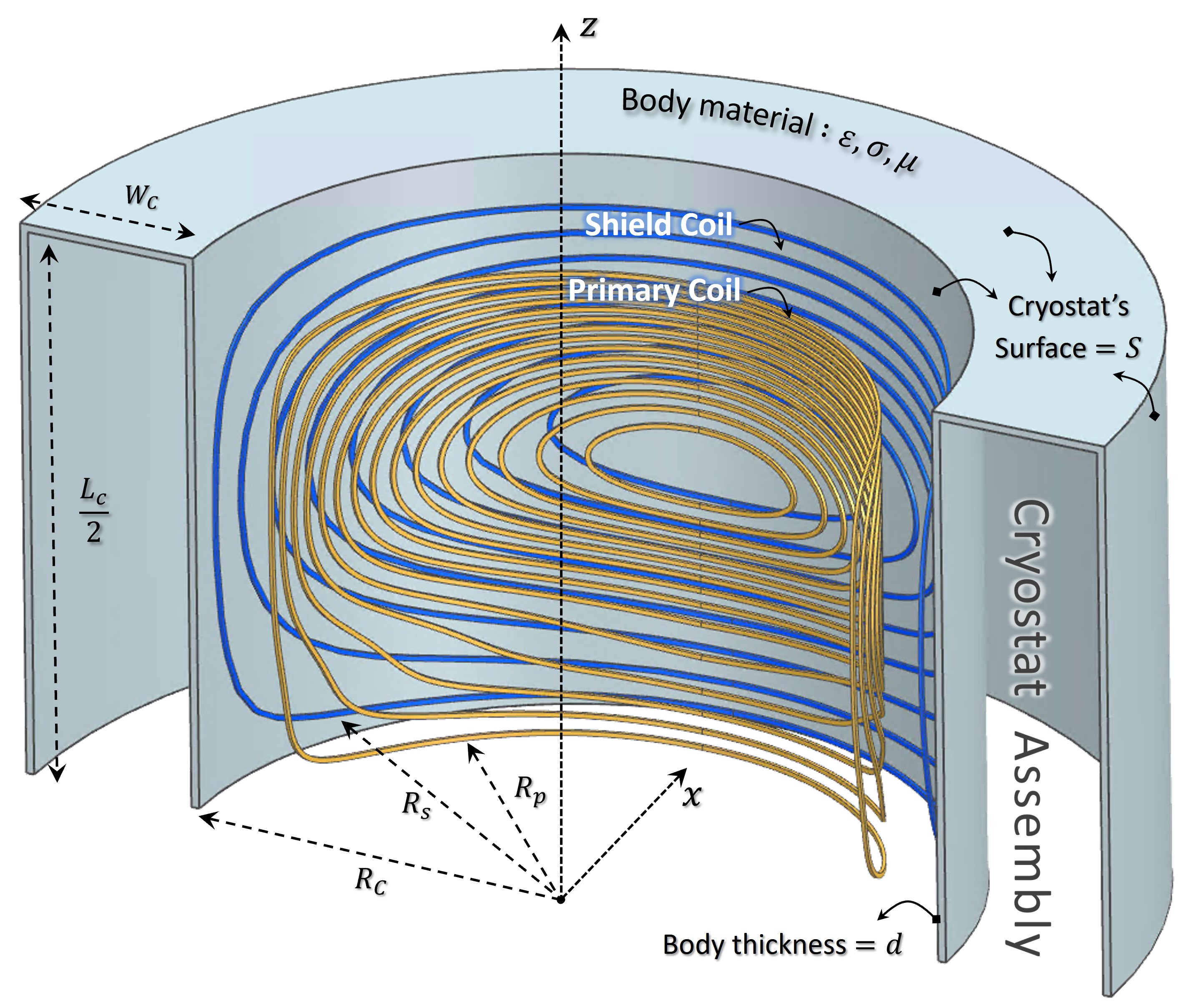
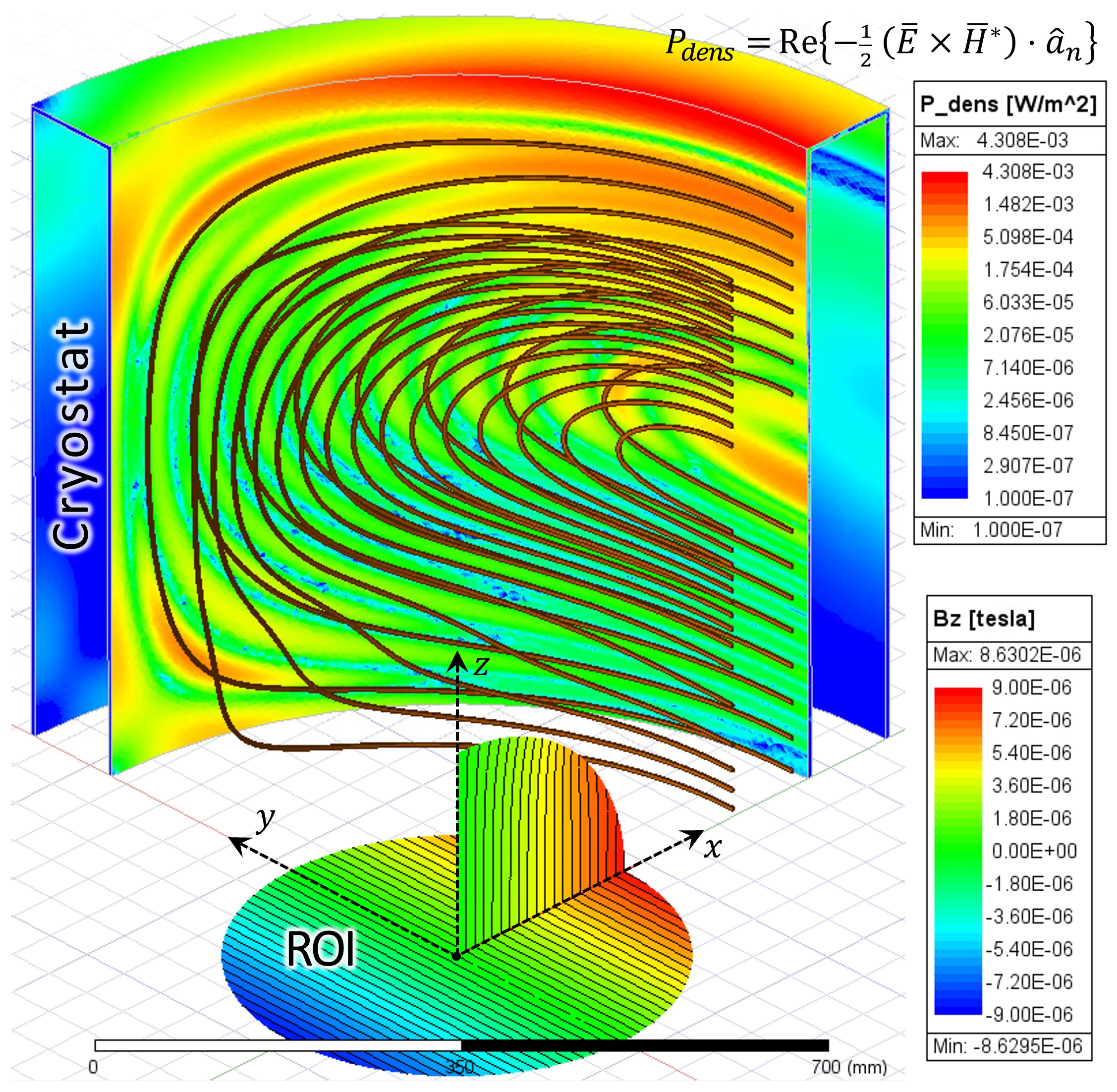
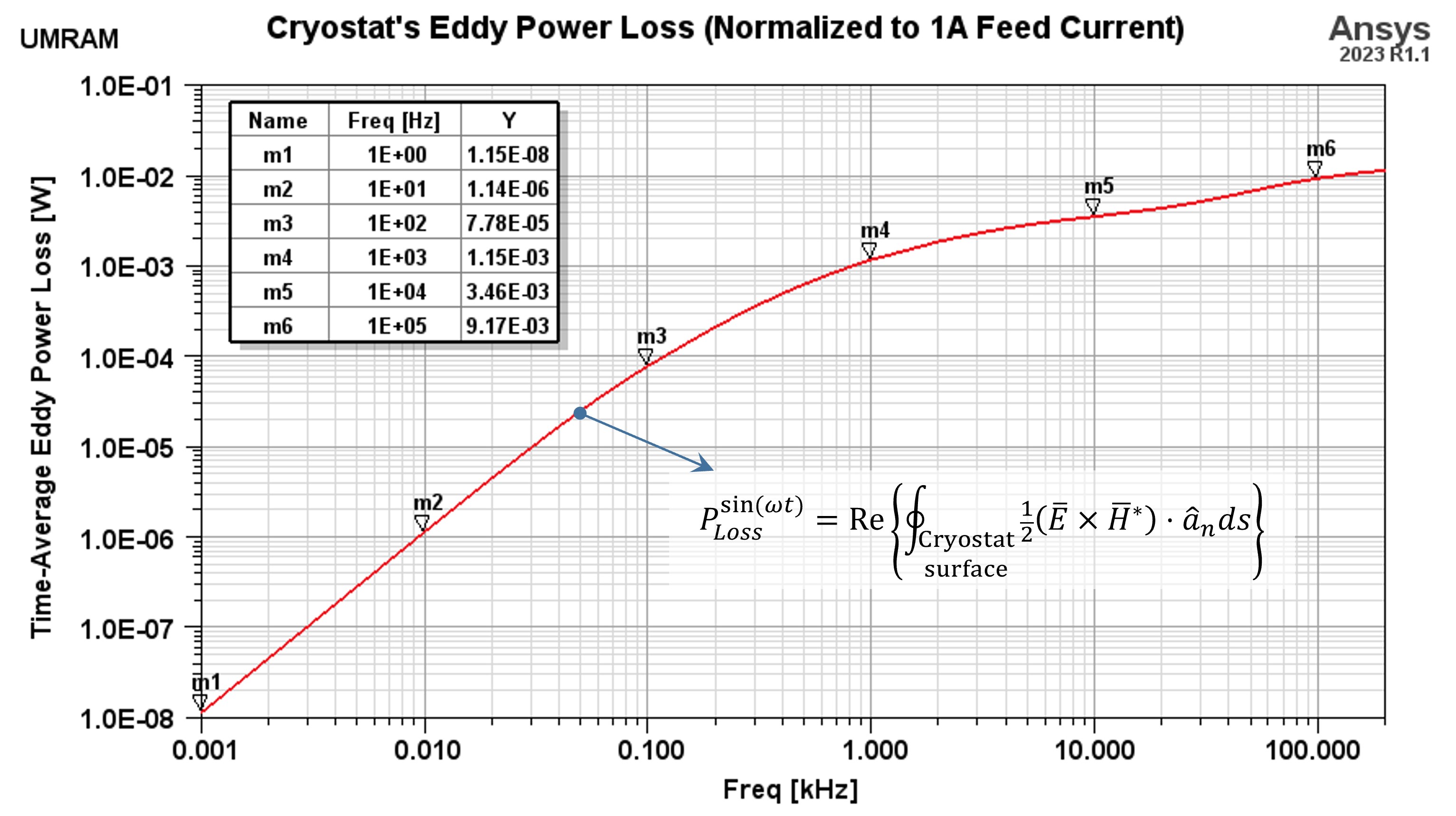
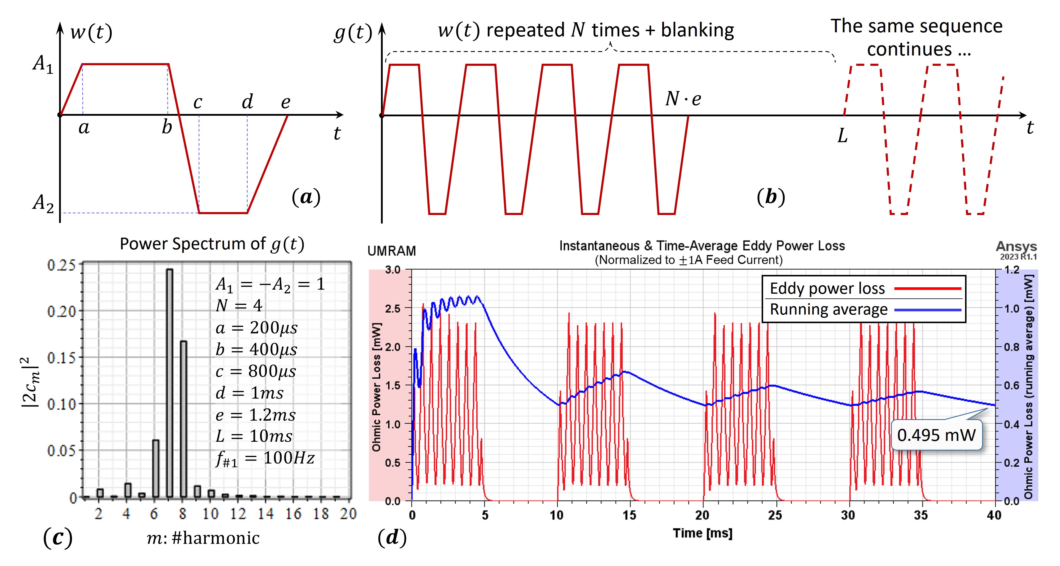
An Intel Xeon® Dell workstation of 128GB memory, Sym4Life 7.0, Maple¹⁰ 2023, and Ansys Maxwell¹¹ 2023 are utilized for coil design, numerical calculations, and field simulations, respectively. Figure 1 illustrates a quarter of a typical 40mT/m whole-body x-gradient coil and a 5mm thick stainless-steel cylindrical cryostat (without internal components for simplicity). Dimensions and parameters are given in the caption. The simulated EM fields, driven by a unity amplitude sinusoidal current, are captured on the cryostat’s surface for a limited range of frequencies concerned with gradient feeding. Figure 2 shows $$$\text{Re}\left\{\!-\frac{1}{2}{\left(\overline{E}\!\times\!\overline{H}^{\,*}\right)\!\cdot{\hat{a}_n}}\right\}$$$, the density of transferred ohmic power per unit area through the cryostat’s surface [W/m²], and $$$B_z$$$, the longitudinal flux density inside the ROI [tesla] at 1kHz.
Field values are imported to Maple for integration and then spline curve fitting. Figure 3 depicts $$$P_{Loss}^{\sin(\omega{t})}(f)$$$ versus frequency. We use a bipolar trapezoidal pulse sequence of 400µs rise/fall time and 200µs plateau time, repeated every 10ms, as shown in Figures 4(a,b). Figure 4(c) shows $$$|2c_m|^2$$$ as the power spectrum of the pulse sequence. Our approach based on Equation [2] reports 0.51mW normalized total power loss. Figure 4(d) illustrates the transient simulation showing the instantaneous eddy power loss within the cryostat (and its running average) for 40ms. Ansys simulation reads 0.495mW, which is about 3% lower and agrees well with the proposed method.

Discussion

Although peak eddy power loss deals with instant heat dissipation, which is vital for handling high loads on occasion, the emphasis is on time-average eddy power loss, which indicates average heat dissipation over time and must be kept low to ensure stable cryogenic temperatures. Our method, utilizing one-time electromagnetic simulations and Fourier transform of the pulse sequence, accurately predicts the total time-average eddy power loss caused by gradient assembly.

Conclusion

We propose a new computational method for calculating time-average eddy power loss in a cryostat given a pulse sequence and coil structure. This approach has three significant advantages: (a) It evaluates power losses throughout the cryostat body, not just the inner surface; (b) its accuracy matches commercial software results; and (c) it can be applied to array/conventional gradient coils of any shape.

Acknowledgements

This work is fully funded by the Scientific and Technological Research Council of Turkey (TÜBİTAK) under Grant No. 121E128. Additionally, the authors acknowledge Sim4Life by ZMT (www.zurichmeditech.com) for providing an Academic License.

References

1. Liu F, Crozier S. An FDTD model for calculation of gradient-induced eddy currents in MRI system. IEEE Trans Appl Supercon. 2004;14:1983-1989.

2. Trakic A, Wang H, Liu F, Lopez HS, Crozier S. Analysis of transient eddy currents in MRI using a cylindrical FDTD method. IEEE Trans Appl Supercon. 2006;16:1924-1936.

3. Trakic A, Liu F, Lopez HS, Wang H, Crozier S. Longitudinal gradient coil optimization in the presence of transient eddy currents. Magn Reson Med. 2007;57(6):1119-1130. doi:10.1002/mrm.21243.

4. Li X, Xia L, ChenW, Liu F, Crozier S, XieD. Finite element analysis of gradient z-coil induced eddy currents in a permanent MRI magnet. J Magn Reson. 2011;208:148-155.

5. Sanchez Lopez H, Freschi F, et al. Multilayer integral method for simulation of eddy currents in thin volumes of arbitrary geometry produced by MRI gradient coils. Magn Reson Med. 2014;71:1912-1922.

6. Sanchez Lopez H, Poole M, Crozier S. Eddy current simulation in thick cylinders of finite length induced by coils of arbitrary geometry. Journal of Magnetic Resonance. 2010;207(2):251-261. doi:10.1016/j.jmr.2010.09.002.

7. Alsharafi SS, Badawi AM, El-Sharkawy AE-MM. Eddy currents analysis methods for an MRI longitudinal gradient coil. Magn Reson Med. 2023;1-17. doi:10.1002/mrm.29777.

8. Takrimi M and Atalar E. A Novel Method to Estimate and Control the Eddy Power Loss within the Cryostat: A Co-Simulation Approach to Tune Z-Gradient Array Coil. In Proceedings of the Joint Annual Meeting of ISMRM & ISMRT. Toronto, 2023: Abstract# 4573.

9. Jackson, John David. Classical Electrodynamics, 3rd ed. Wiley, 1999.

10. Maple 2022. Maplesoft, a division of Waterloo Maple Inc., Waterloo, Ontario.

11. https://www.ansys.com/products/electronics. Accessed Sep 10, 2023.

Figures

Figure 1: The cross-section view of a quarter of a simplified cylindrical cryostat assembly made of stainless steel and a whole-body x-gradient coil consisting of both the primary and shield coils made of copper. The coil is designed by Sim4Life for 5% linearity and 45cm diameter of spherical region. Cryostat parameters are: length L_C=1.4 m, inner radius R_C=47 cm, end plate width W_C=10 cm, thickness d=5 mm, and conductivity 1.39 MS/m. X-gradient coil dimensions are: R_P=37 cm, R_S=45 cm. The inner components of the cryostat assembly are neither considered nor simulated for simplicity.

Figure 2: Different field plots for half of the configuration shown in Figure 1 with unity amplitude sinusoidal excitation at f=1 kHz. The 5.5% field linearity for the longitudinal magnetic flux density B_z is shown inside the 45 cm diameter ROI. Additionally, P_dens, the density of the transferred ohmic power [W/m²] is shown on all surfaces of the cryostat body.

Figure 3: The total time-average eddy power loss P_Loss^sin(wt) on the cryostat’s surface, driven by a sinusoidal current of unity amplitude, is plotted against frequency. Markers m1 to m6, listed in the table, represent a few power loss values for a five-order-of-magnitude change in frequency.

Figure 4: (a) w(t) is a bipolar trapezoidal pulse of amplitudes A₁,A_2, and breakpoints a,b,c,d,e. (b) The feeding current g(t) is an N times repeated version of w(t), followed by a blank signal that extends up to t=L and then repeats indefinitely. (c) Power spectrum of g(t) for N=4, a=200 μs, b=400 μs, c=800 μs, d=1 ms, e=1.2 ms, and L=10 ms. (d) Four cycles of the transient simulation showing the instantaneous eddy power loss (and its running average) for 40 ms. The Ansys transient simulation reads 0.495 mW, which is about 3% lower and agrees well with the proposed method.

Proc. Intl. Soc. Mag. Reson. Med. 32 (2024)

3913

DOI: https://doi.org/10.58530/2024/3913