3688
A Joint 2.5D Physics-coupled Deep learning based Polynomial Fitting Approach for MR Electrical Properties Tomography1Department of Electrical and Electronic Engineering, Yonsei Univeristy, Seoul, Korea, Republic of, 2Department of Radiotherapy, UMC Utrecht, Utrecht, Netherlands, 3Computational Imaging Group for MR Therapy and Diagnostics, UMC Utrecht, Utrecht, Netherlands, 4Department of Radiology, Gangnam Severance Hospital, Yonsei University College of Medicine, Seoul, Korea, Republic of
Synopsis
Keywords: Electromagnetic Tissue Properties, Electromagnetic Tissue Properties
Motivation: Conductivity reconstructions based on polynomial fitting methods are mostly 2D leading to inaccurate reconstructions as information arising from the through-plane dimension is missing.
Goal(s): To include conductivity contributions from three-dimensions for deep-learning patch-based polynomial fitting reconstructions.
Approach: A DL-informed polynomial fitting reconstruction method including $$$B_{1}^{+}$$$ magnitude information is presented. This method leverages neural networks to jointly predict optimal fitting coefficients enabling joint 2D-polynomial-fitting in three-orthogonal-planes, hence we call it 2.5D.
Results: The proposed method demonstrates superior-performance compared to fitting-based 2D/3D fitting approaches and is computationally efficient for 3D-reconstructions.
Impact: A 2.5-dimensional neural network informed fitting approach is used for MR-based conductivity reconstructions. Conductivity reconstruction accuracy as well as structural information are improved compared to physics-based and deep learning-based fitting methods.
Introduction
Electrical Properties Tomography (EPT) reconstructs tissue conductivity (σ) from $$$B_{1}^{+/-}$$$ fields. Fitting-based methods have been presented as good candidates to mitigate noise amplification inherent in Helmholtz-based methods1,2,3,4. To minimize errors at tissue-boundaries, these methods employ weights derived from MRI-contrast5,6,7. Recently, deep learning (DL)-informed approach has shown good potential in determining weights without the need for segmentation8(2D DL-Fit).However, these are 2D reconstruction methods, thus conductivity information arising from phase variations in third-dimension (slice-direction) is neglected. Additionally, these methods do not consider $$$\left| B_1^+ \right|$$$ information.
We present a DL-informed fitting reconstruction method, including the $$$B_{1}^{+}$$$ magnitude, and utilizes information from all three-planes (axial/coronal/sagittal). This method leverages three neural networks to jointly predict optimal fitting coefficients enabling joint 2D-polynomial-fitting in three-orthogonal-planes, hence we call it 2.5D. The method is tested on simulated and measured data.
Method
In polynomial fitting approaches, the conductivity is inferred from the measured phase curvature approximated with second-order polynomials with β-coefficients. The fitting process is refined using weights to account for signal magnitude variations, yielding to optimized β-coefficients that minimize the impact of noise and errors at tissue interfaces(Poly-Fit)6. These β-coefficients are computed using:$$\hat{\beta} = \left( M^TWM \right)^{-1}M^TWP \tag{1}$$
With M=Vandermonde matrix, W=diagonal matrix with fitting weights, P=phase vector. 2D in-plane tissue conductivity is then computed as:
$$\sigma = \frac{2 \cdot (\hat{\beta}_5 + \hat{\beta}_6)}{\mu_0 \omega} \tag{2}$$
Incorporating $$$\left| B_1^+ \right|$$$, with $$$\alpha = \ln\left( \left| B_1^+ \right| / M \right)$$$, Eq.2 becomes:
$$\sigma = \frac{2 (\hat{\beta}_5 + \hat{\beta}_6)}{\mu_0 \omega} + \frac{2 (\hat{\beta}_2 \hat{\alpha}_2 + \hat{\beta}_3 \hat{\alpha}_3)}{\mu_0 \omega} \tag{3}$$
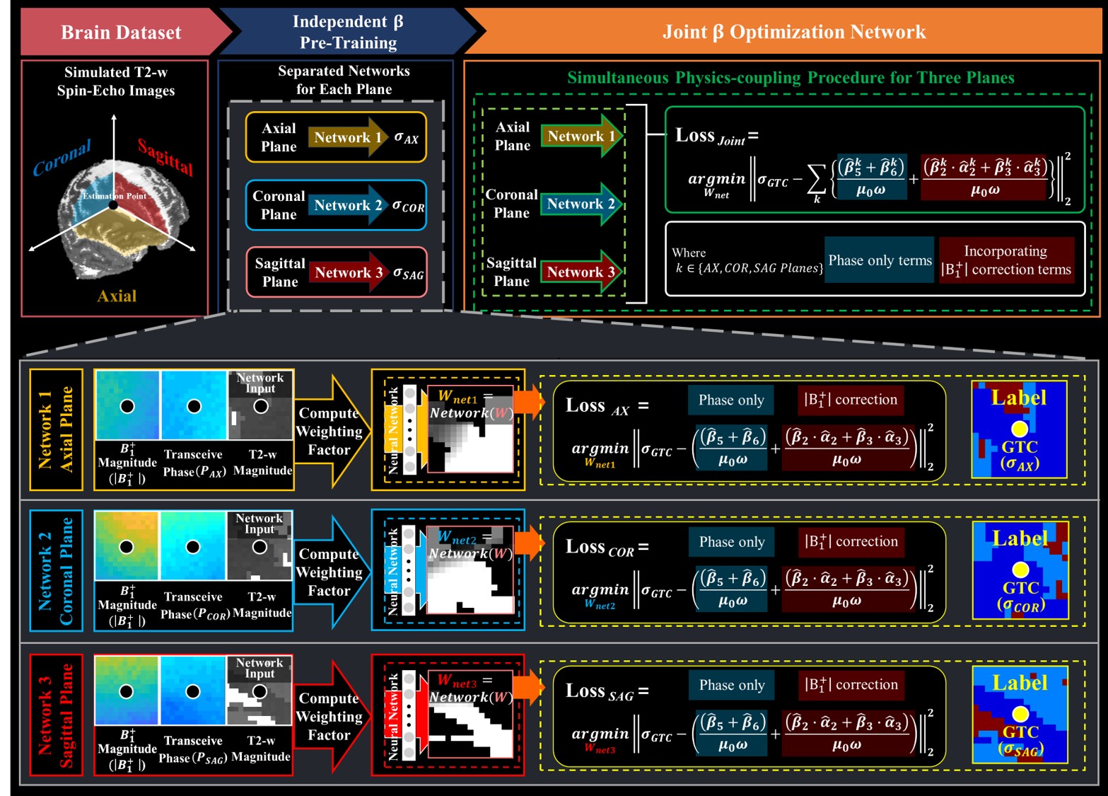
Previously, the weights W were computed only in-plane. Here, we extend this to 3D as 3x2D orthogonal planes. Firstly, three patch-based(15X15 voxels) networks are independently trained to compute optimal β-coefficients for each 2D plane (βAX,βCOR, and βSAG) (Fig.1: Independent pre-training). From this, conductivity maps are calculated in accordance with Eq.3. Then, a joint optimization process10 is performed by integrating the physics-relationship of independently pre-trained network weights from each plane(Fig.1: Joint optimization network). The final loss function aims to combine the information from the 3x2D-planes as:
$$\text{Loss}_{\text{Joint}} = \arg\min_{W_{\text{net}}} \left\| \sigma_{\text{GTC}} - \sum_{k} \left( \frac{(\hat{\beta}_5^k + \hat{\beta}_6^k)}{\mu_0 \omega} + \frac{(\hat{\beta}_2^k \cdot \hat{\alpha}_2^k + \hat{\beta}_3^k \cdot \hat{\alpha}_3^k)}{\mu_0 \omega} \right) \right\|_2^2 \text{ where } k \in \{\text{AX}, \text{COR}, \text{SAG}\}\text{-planes} \tag{4}$$
For training, 15 different brain models with different EP values and tumor inclusions were used9. $$$B_{1}^{+}$$$ complex fields were simulated in Sim4Life from which the transceive phase was computed11,12 (ZMT, Zurich, Switzerland). The optimization of the β-coefficients was performed by minimizing the L2 loss between the ground-truth and the predicted conductivity. The details of the workflow are depicted in Fig.1.
Overall training time was 14 hours. Testing was performed on: 1) simulated healthy brain model (noiseless and with noise, SNR=40) and tumor brain model (SNR=40); 2) a healthy volunteer (TSE,3T,Philips,Ingenia); 3) a brain tumor patient (TSE,3T,GE,MR750).
Results and Discussion
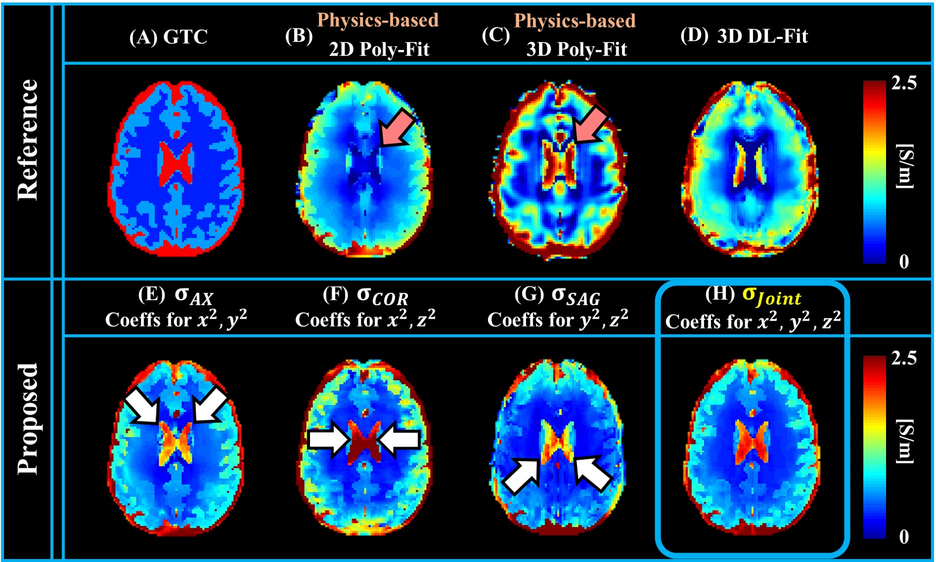
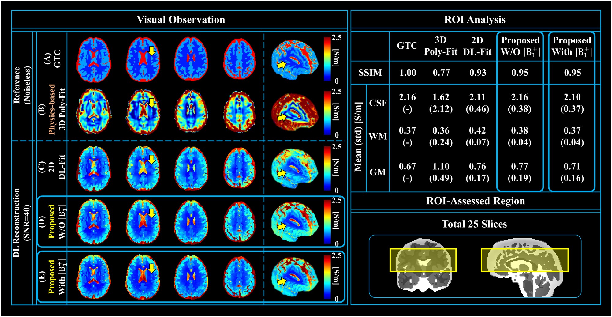
In Fig.2, the results of the proposed method are presented for a brain model without noise. The results with physics-based Poly-Fit(B,C) are displayed to demonstrate the impact of z-variation (pink-arrows) and compared to our 2.5D method(H). The white-arrows(E,F,G) highlight the different conductivity contributions arising from 2D reconstructions for each plane independently. Just as an example, directly utilizing 3D kernel resulted in inferior performance(D).In Fig.3, 3D physics-based, 2D DL-Fit, and 2.5D DL-Fit (with/without $$$\left| B_1^+ \right|$$$) reconstructions on a simulated brain model with SNR=40 are compared. The proposed method demonstrates higher accuracy (see ROI analysis) and better captures the fine details of structural information (yellow-arrows).
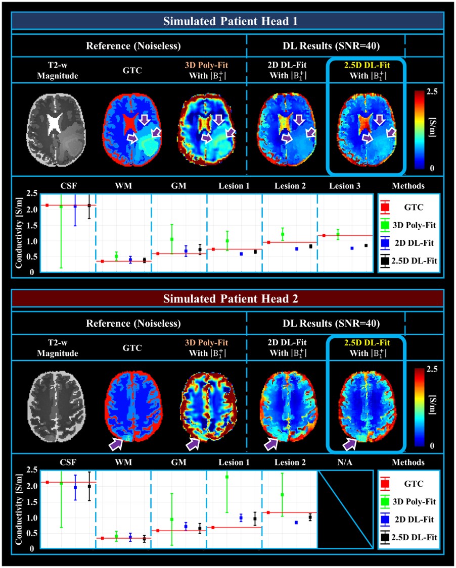
In Fig.4, 3D physics-based Poly-Fit, 2D DL-Fit and 2.5D DL-Fit (with $$$\left| B_1^+ \right|$$$) reconstructions on two tumor models are compared. The tumor is clearly visible in the proposed reconstructions and shows better homogeneity compared to reference methods (Fig.4 ROI Analysis Graph).
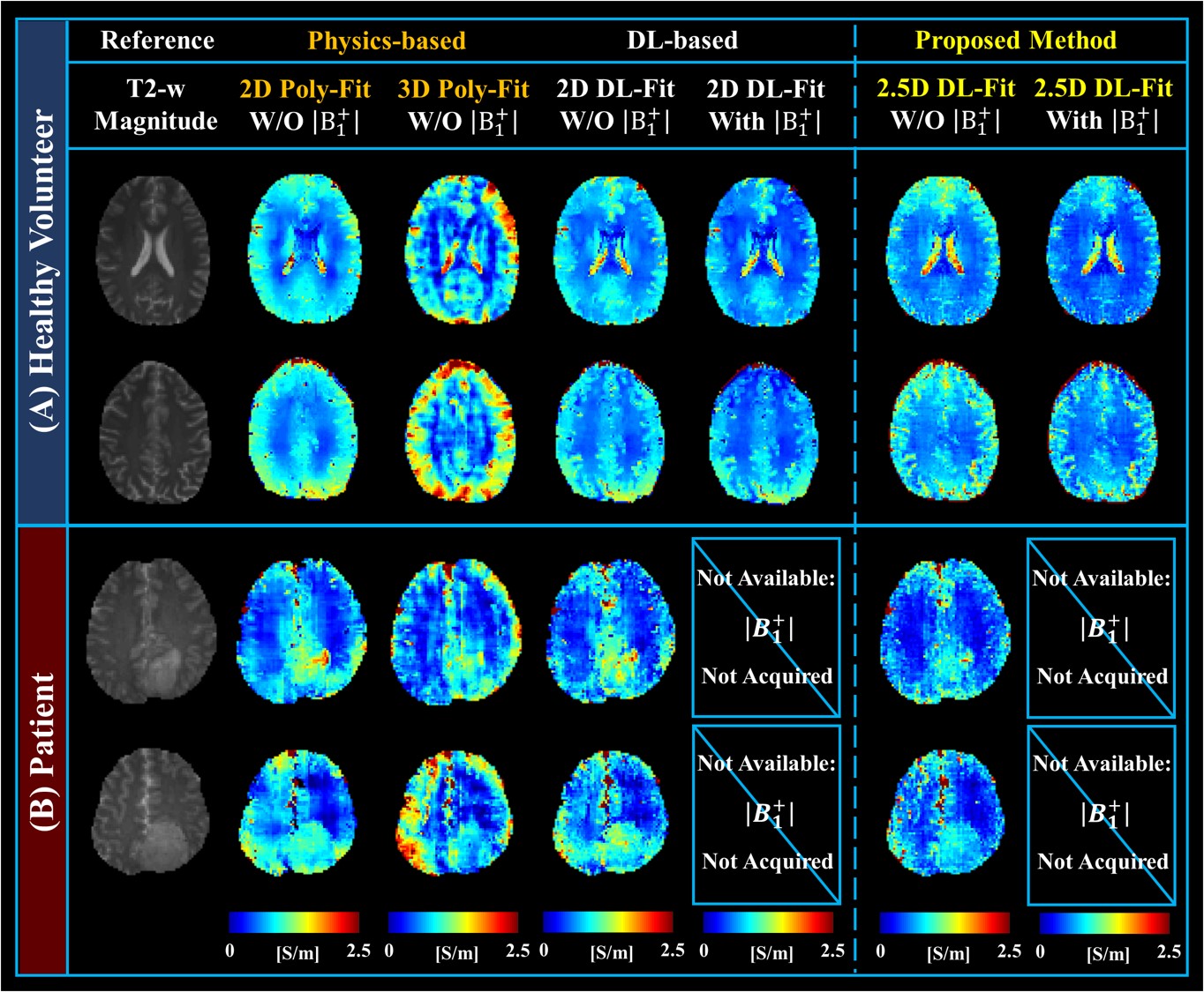
In Fig.5 reconstructions on a healthy volunteer and tumor patient show that the proposed method produces realistic results in-vivo in 4 minutes 30 seconds for 80 slices, with higher quality than other reconstruction methods used as references.
Overall, the 2.5D physics-coupled network refines reconstructions by exclusively adjusting fitting coefficients, thereby preserving physics-based reconstructions of conductivity. This method efficiently computes joint 2.5D reconstructions, considering the z-variation $$$\left| B_1^+ \right|$$$ and transceive phase. This significantly reduces reconstruction errors relative to two-dimensional methods. The inclusion of $$$\left| B_1^+ \right|$$$ also reduced the erroneous increase in conductivity values at the periphery of the brain, typical of phase-only methods.
Conclusion
We have introduced a 2.5D DL-Fit method that incorporates a physics-informed tri-plane approach to include conductivity variations from 3-dimensions. This method outperforms physics-based Poly-Fit and 2D DL-Fit methods. Furthermore, our method optimizes computational efficiency for 3D reconstructions.Acknowledgements
The first two authors share first authorship, while the last two authors share last authorship.
This work received funding from the Netherlands Organization for Scientific Research (NWO; VENI grant no. 18078), the Artificial Intelligence working group of the EWUU alliance; and the ISMRM research exchange program.
This work has been supported by Y-BASE R&E Institute, a Brain Korea 21 four program, Yonsei University.
References
[1] Katscher U, et al., Determination of Electric Conductivity and Local SAR Via B1 Mapping. IEEE transactions on medical imaging, 2009;28(9):1365-1374.
[2] Voigt T, et al., Quantitative conductivity and permittivity imaging of the human brain using electrical properties tomography. Magnetic Resonance in Medicine, 2011;66(2):456-466.
[3] Leijsen, R., Brink, W., van den Berg, C., Webb, A., & Remis, R., Electrical properties tomography: A methodological review. Diagnostics, 2021;11(2): 176.
[4] Mandija, S., et al., Error analysis of helmholtz‐based MR‐electrical properties tomography. Magnetic Resonance in Medicine, 2018;80(1): 90-100.
[5] Katscher, U., et al., Estimation of Breast Tumor Conductivity Using Parabolic Phase Fitting. ISMRM 20th Annual Meeting, 5-11 May 2012.
[6] Lee J, et al. MR‐based conductivity imaging using multiple receiver coils. Magnetic Resonance in Medicine, 2016;76(2):530-539.
[7] Karsa, A., & Shmueli, K. New Approaches for Simultaneous Noise Suppression and Edge Preservation to Achieve Accurate Quantitative Conductivity Mapping in Noisy Images. ISMRM 29th Annual Meeting, 15-20 May 2021.
[8] Jung, K-J., et al, K. A Deep learning Informed Polynomial Fitting Approach for Electrical Properties Tomography. 2023 ISMRM Annual Meeting, 3-8 June 2023.
[9] Meerbothe, T.G., et al., Electrical properties tomography: A database for MR-based electrical properties tomography with in silico brain data-ADEPT, Magnetic Resonance in Medicine, 2023; Online Published.
[10] Nguyen, A., et al., Plug & play generative networks: Conditional iterative generation of images in latent space, CVPR 2017, 21-26 July 2017: 4467-4477.
[11] Christ, A., et al., The virtual family—Development of surface-based anatomical models of two adults and two children for dosimetric simulations, Physics in Medicine & Biology, 2009;55(2): N23-N38.
[12] Gosselin, M.C., et al., Development of a new generation of high-resolution anatomical models for medical device evaluation: The virtual population 3.0, Physics in Medicine & Biology, 2014;59(18): 5287-5303.
Figures