3684
2D vs 3D Electrical Properties Tomography reconstruction: The impact of disregarding the third dimension.1Department of Radiotherapy, Division of Imaging and Oncology, University Medical Center Utrecht, Utrecht, Netherlands, 2Computational Imaging Group for MR Therapy and Diagnostics, University Medical Center Utrecht, Utrecht, Netherlands, 3Department of Electrical and Electronic Engineering, Yonsei University, Seoul, Korea, Republic of
Synopsis
Keywords: Electromagnetic Tissue Properties, Electromagnetic Tissue Properties, Conductivity, EPT
Motivation: In Electrical Properties Tomography, often 2D reconstructions ignoring derivatives in the slice direction (often z) are performed instead of 3D reconstructions, without proper compensation.
Goal(s): In this work, we investigate the quantitative influence on the reconstructed conductivity.
Approach: This is done by experiments in a cylindrical phantom with homogeneous electrical properties in simulation and measurement. Furthermore, using simulations an indication is given of the importance of 3D reconstruction in several anatomical areas.
Results: The contribution of the third dimension on the reconstructed conductivity is shown to be highly dependent on sample geometry. Therefore, disregarding this can only be done in specific cases.
Impact: This work shows that the assumption of a negligible third dimension contribution as done in 2D EPT reconstruction is only accurate in specific cases. For most applications 3D reconstructions or proper compensation is needed.
Introduction
In Electrical Properties Tomography (EPT), tissue conductivity (σ) can be reconstructed by taking spatial derivatives of the measured radiofrequency, B1+ field in the x, y, and z directions1.However, this is often done in 2D (in-plane), disregarding the spatial variation of the B1+ field from the slice direction (often the z-direction) because of: 1) the use of 2D acquisitions, 2) a contribution to the conductivity from z-curvature of the B1+ field is considered to be negligible2; leading to errors in reconstructed conductivity. Compensation is possible under the assumption that all spatial dimensions contribute equally to the conductivity3. Although these assumptions can hold in specific situations, the influence of the third direction is generally unknown and dependent on the sample geometry4.
In this study, we quantify the contribution of the third dimension to the conductivity in the case of a homogeneous cylindrical phantom, measured and simulated. Additionally, by means of simulated data, we give an indication of this contribution for several anatomical areas.
Methods
For piece-wise constant electrical properties, the conductivity can be reconstructed using the homogeneous Helmholtz equation1:$$\frac{1}{\mu_0\omega}Im\bigg\{\frac{\frac{\partial^2B_1^+}{\partial{x^2}}}{B_1^+}+\frac{\frac{\partial^2B_1^+}{\partial{y^2}}}{B_1^+}+\frac{\frac{\partial^2B_1^+}{\partial z^2}}{B_1^+}\bigg\}=\sigma_x+\sigma_y+\sigma_z$$
with µ0=vacuum permeability, ω=Larmor frequency and σx,y,z is the conductivity contribution from each spatial direction. However, depending on the sample dimensions, the ratio of σx,y,z/σ may differ.
To assess the impact of σz, MRI experiments were done on a 3 T MRI (Ingenia, Philips) using a cylindrical gelatin-based phantom with σ=0.6 S/m, constant radius r, and variable length L obtained by cutting the cylinder to reduce length. Each cylinder, with different ratios r/L, was scanned in transverse orientation (slice direction z=Feet-Head), while keeping the mid-plane at the same location within the MRI bore. The experiment was reproduced in simulations (Sim4Life, ZMT)7. Measurement and simulation details are displayed in Figure 1.
Polynomial fitting was used for conductivity reconstructions8, including |B1+| information. This was done with a kernel size 21x21x21 for MRI data to overcome noise effects and kernel size 5x5x5 for simulated data.
First, the measured and simulated B1+ magnitude and transceive phase (approximating the transmit phase9) were compared to validate the simulated setup. Then, for all simulated and measured cylinder phantoms, 2D and 3D conductivity reconstructions were done to assess the contribution of σz to the total conductivity when varying the r/L ratio.
Finally, we estimated the contribution of σz for different body parts of Duke (leg, heart, brain, prostate and ventricles)10 from noiseless simulated data, to conduct preliminary investigations for future studies on such anatomical areas.
Results and discussion
Figure 2 shows very good agreement between the measured and simulated B1+ fields for a cylinder of length 119 mm (r/L=0.5), demonstrating the validity of the simulation setup.Figure 3 shows a good agreement between 2D/3D conductivity reconstructions from MRI and simulated data for the different cylinder lengths. While 3D reconstructions show similar conductivity values for decreasing cylinder lengths, 2D reconstruction show a clear decrease in conductivity values. This indicates that σz has a larger relative contribution for a shorter cylinder. Simulation results show that this effect is spatially dependent; it is lower when moving radially from the center to the sides of the phantom. This is less evident for conductivity reconstructions from MRI data due to banding artifacts corrupting the reconstructions near the edges and the large reconstruction kernel dealing with noise.
Figure 4 shows a linear relation between the relative σz contribution and the ratio r/L, for both MRI and simulated data. For this geometry, σz is negligible when L>4r, while σz has the largest relative contribution for L<2r.
Figure 5 shows an indication of σz contribution for different body parts. For a leg, cylindrically shaped with (r<<L), the z-contribution is small. Organs with more spherical dimensions (r≈L) such as the heart, brain white matter and the prostate, have σz contributions up to 50 %. Ventricles, with orientation such that r>>L show very high σz contribution. This indicates the importance of including σz.
These experiments show that the σz contribution is geometry dependent and cannot be easily disregarded. However, this investigation only deals with a single compartment phantom with piece-wise constant conductivity. Future research should therefore focus on analyzing the σz contribution in a multi-compartment scenario, with tissues of different electrical properties.
Conclusion
This investigation has shown that for a homogeneous cylinder, σz is linearly dependent on the fraction of r/L and that σz is very dependent on the sample geometry. Thus, σz cannot simply be disregarded if the studied geometry in z is not significantly larger than x and y.Acknowledgements
This work received funding from the Netherlands Organization for Scientific Research (NWO; VENI grant no. 18078), the Artificial Intelligence working group of the EWUU alliance; and the ISMRM research exchange program.References
[1] Leijsen R, Brink W, van den Berg CAT, Webb A, Remis R. Electrical properties tomography: A methodological review. Diagnostics. 2021. 11(2), 176. doi: 10.3390/diagnostics11020176.
[2] Hafalir FS, Oran OF, Gurler N, & Ider YZ (2014). Convection-reaction equation based magnetic resonance electrical properties tomography (cr-MREPT). IEEE transactions on medical imaging, 33(3), 777-793.
[3] Katscher U, & Weiss S. (2022). Mapping electric bulk conductivity in the human heart. Magnetic Resonance in Medicine, 87(3), 1500-1506.
[4] Lee J, Choi N, Seo JK, Kim DH. Magnetic resonance electrical properties tomography for small anomalies using boundary conditions: A simulation study. Med Phys. 2017 Sep;44(9):4773-4785. doi: 10.1002/mp.12343. Epub 2017 Aug 22. PMID: 28508476.
[5] Hampe N, Katscher U, van den Berg CAT, Tha KK, Mandija S. Deep learning brain conductivity mapping using a patch-based 3D U-net. arXiv preprint. 2019. doi: 10.48550/arXiv.1908.04118.
[6] Yarnykh VL. Actual flip-angle imaging in the pulsed steady state: a method for rapid three-dimensional mapping of the transmitted radiofrequency field. Magnetic Resonance in Medicine: 2007. doi: 10.1002/mrm.21120
[7] Meerbothe TG, Meliado EF, Stijnman PRS, van den Berg CAT, Mandija S. A Database for MR-based Electrical Properties Tomography with in silico brain data – ADEPT, Magn Reson Med. 2023; 1-10. doi: 10.1002/mrm.29904
[8] Karsa, A., & Shmueli, K. New Approaches for Simultaneous Noise Suppression and Edge Preservation to Achieve Accurate Quantitative Conductivity Mapping in Noisy Images. ISMRM 29th Annual Meeting, 15-20 May 2021
[9] van Lier AL, Raaijmakers A, Voigt T, Lagendijk JJ, Luijten PR, Katscher U, van den Berg, C A. Electrical properties tomography in the human brain at 1.5, 3, and 7T: a comparison study. Magn Reson Med. 2014. 71(1), 354-363. doi: 10.1002/mrm.24637
[10] Christ A. et al. "The Virtual Family—development of surface-based anatomical models of two adults and two children for dosimetric simulations." Physics in Medicine & Biology. 55, 23–38 (2010).
Figures
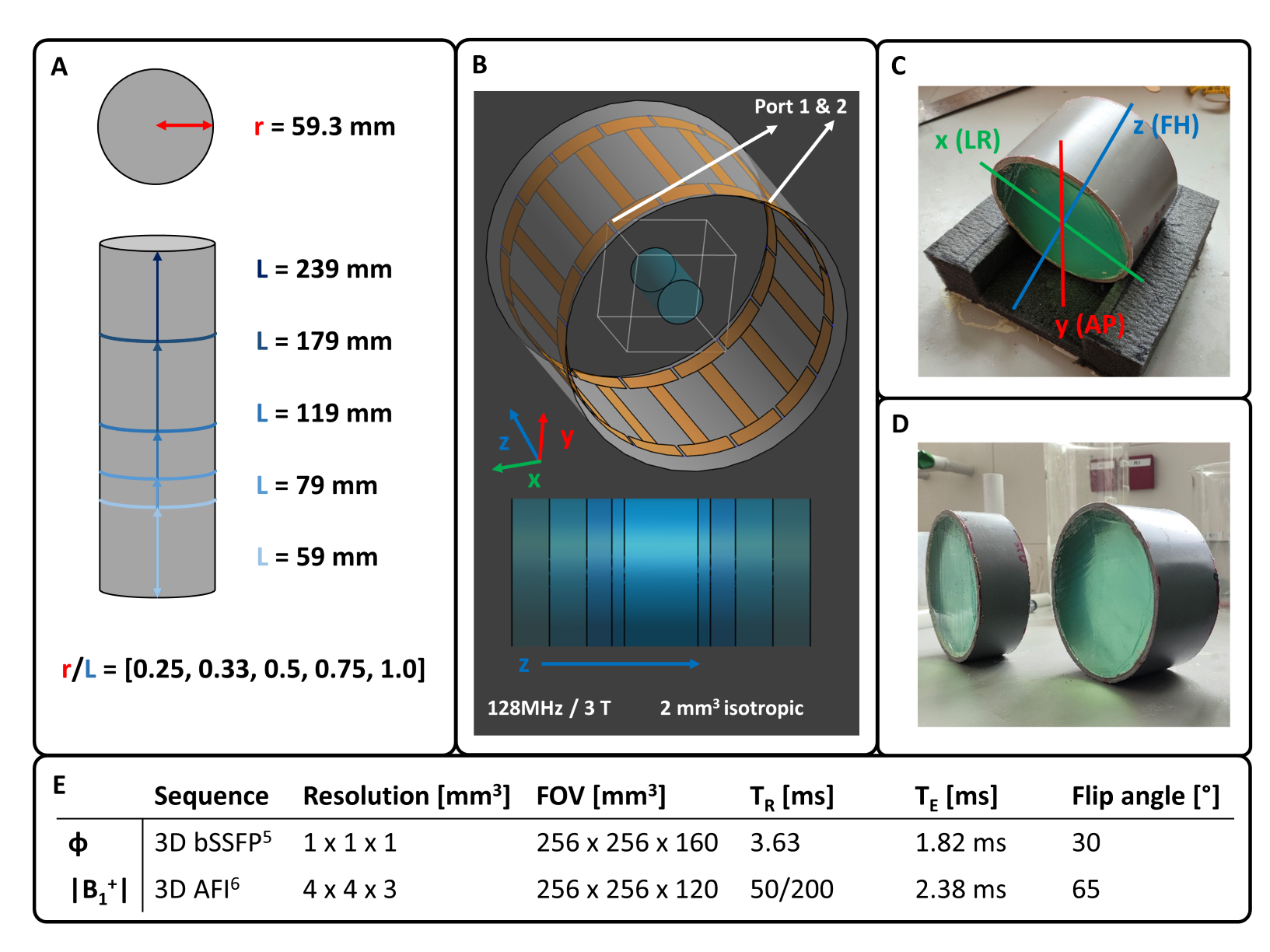
Figure 1: Measurement and simulation setup. A: Schematic view of the cylinder phantom with different lengths. B: Simulation setup of different sized cylinders within the coil in Sim4Life. C: Cylinder in foam holder, which is placed inside the MRI. D: Example of two cylinders cut in different lengths. E: Measurement sequence parameters.
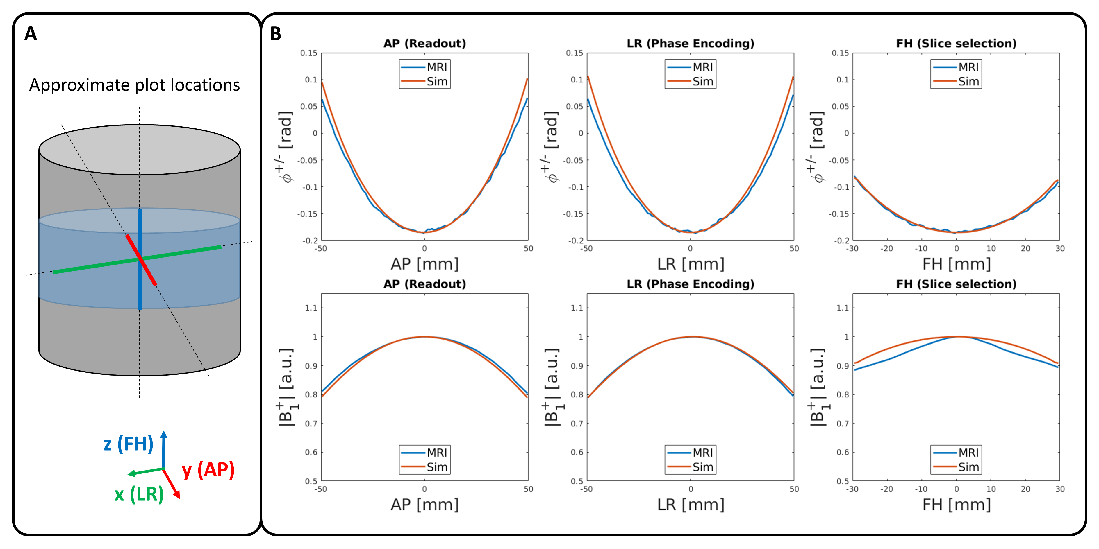
Figure 2: Validation of the simulation setup for a cylinder length of 119 mm (r/L = 0.5), with a comparison between the simulated and measured fields in all directions. A: approximate locations of the plotted lines. B: Comparison of measured and simulated fields.
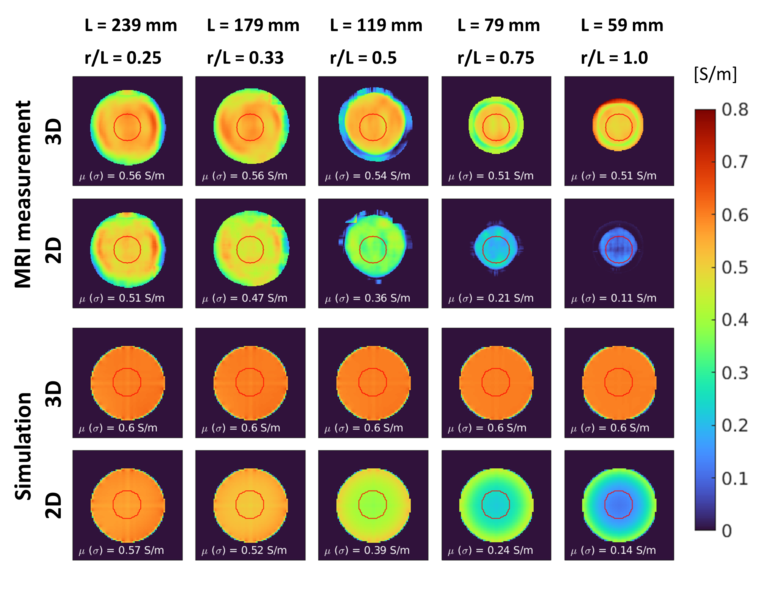
Figure 3: Reconstructed conductivity in 3D and 2D for cylinders of varying length. Top two rows depict reconstructions from MRI data, bottom two rows show reconstructions for simulated data. The 3D reconstructions from simulations are highly similar to the ground truth conductivity map.
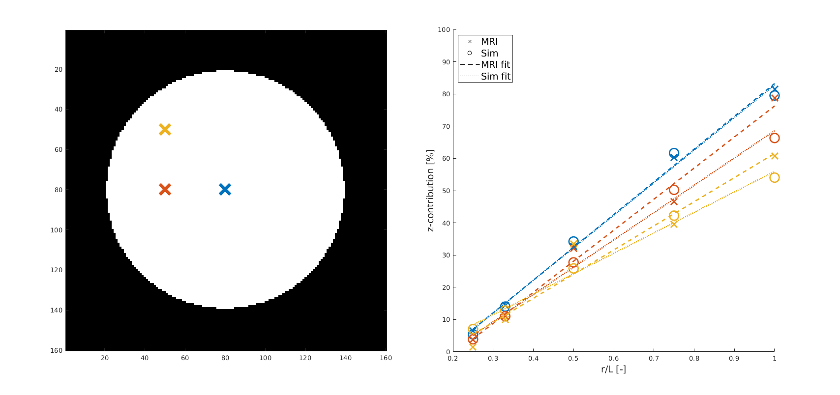
Figure 4: Relative contribution of σz as a function of radius/length is compared for MRI measurements and simulations (right) for three different locations in the center slice of the cylinder (indicated with the crosses on the left). Linear fits on the measurement data display the clear difference of the z-contribution on the different locations.
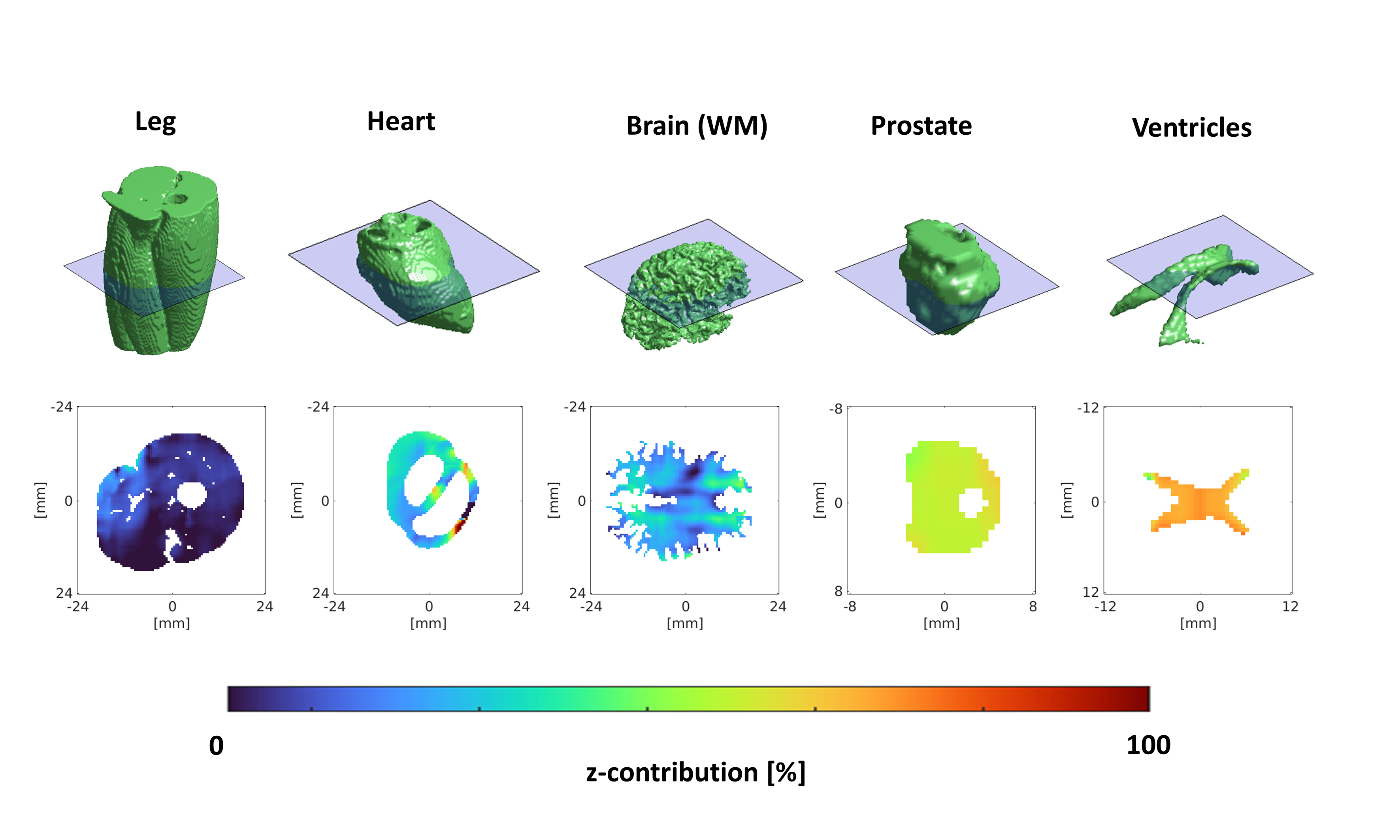
Figure 5: Simulated z-contribution, estimated with large reconstruction kernel for smoother results (21x21x21), in several body parts (bottom row). Corresponding 3D models are displayed in the top row. White voxels are outside of the geometry. Different body parts clearly show big differences in z-contribution