3682

An Automatically Optimised Gaussian Weighting Function Width for Magnitude-Weighted Phase-Based Electrical Properties Tomography (EPT)

Jierong Luo¹, Oriana Arsenov¹, and Karin Shmueli¹
¹Department of Medical Physics and Biomedical Engineering, University College London, London, United Kingdom

Synopsis

Keywords: Electromagnetic Tissue Properties, Electromagnetic Tissue Properties, MR-EPT, electrical conductivity mapping, electrical properties tomography, noise reduction

Motivation: Phase-based electrical properties tomography calculates conductivities by fitting the transceive phase weighted by a Gaussian function of the magnitude image with width δ. Currently, δ is selected empirically and its impact on conductivities is unknown.

Goal(s): To investigate the effect of δ on conductivity maps and develop a method to automatically select δ.

Approach: After evaluating relationships between δ and healthy brain conductivities at 3T, we calculated conductivities using a voxel-wise δ based on inverse phase noise and compared the results.

Results: Increasing δ decreased contrast and noise in conductivity maps. Our new method to calculate a varying δ automatically optimised conductivity maps.

Impact: We have developed a method to calculate a varying Gaussian weighting width for EPT. This will enable automatic optimisation of conductivity maps rather than time-consuming empirical choice of δ, facilitating the use of phase-based EPT and broadening its applicability.

Introduction

Phase-based MR Electrical Properties Tomography (EPT) can calculate tissue conductivities from transceive phase ($$$\phi_{0}$$$) using the integral form of the truncated Helmholtz equation^1-2, via parabolic fitting of $$$\phi_{0}$$$ within a kernel³. Advanced EPT methods can weight the fit with magnitude images^4-6 and refine kernels using magnitude-informed tissue segmentations^{4, 7-8}. These methods better preserve the local homogeneity assumption², and rely on separating different tissue types based on distinguishable Gaussian distributions of magnitude signal intensities^4-6, or using a given threshold^7-8. For magnitude-weighted EPT, the weight $$$W$$$ is often determined by a Gaussian radial basis function of the magnitude as^{4, 6}
$$W=e^{-\frac{(M_{i}-M_{0})^2}{2\delta^2}}$$
where $$$M_{0}$$$ denotes the normalised signal magnitude of the kernel’s central voxel, and $$$M_{i}$$$ denotes the magnitudes of neighbouring voxels within the kernel. The standard deviation $$$\delta$$$ is a free parameter, determining the width of the Gaussian distribution.
In previous magnitude-weighted EPT studies^4-6, the selected $$$\delta$$$ value was seldom reported⁵ or justified⁶, or the selection of $$$\delta$$$ was based on visual inspection^{4, 7-8}. These studies employed a single value of $$$\delta$$$ for all voxels, i.e. a fixed Gaussian distribution, assuming all tissue types have the same magnitude standard deviation. Although a minimal $$$\delta$$$ may guarantee the separation of different tissue types in noiseless or high SNR data⁵, in MRI sequences with lower SNR, a small $$$\delta$$$ can amplify the noise within a tissue type, e.g. a brain region.
Here, we investigated the impact of $$$\delta$$$ on in-vivo brain EPT for the first time. We present a new magnitude-weighted EPT method, using a Gaussian radial basis function with $$$\delta$$$ varying automatically.

Methods

MRI acquisition:
To demonstrate the effect of $$$\delta$$$ in noisy data, multi-echo 2D GRE-EPI was acquired in a healthy volunteer at 3T (Siemens, Prisma) using 64-channel head coil, GRAPPA=4, TR=4034 ms, TEs=15.6, 41.6, 67.6 ms, 1.3 mm isotropic resolution.
EPT:
A non-linear fit⁹ of the complex data over TEs was employed to estimate the field map. We unwrapped the field map using SEGUE¹⁰, and used it to extrapolate the offset at TE=0 ms from the complex data for each TE. $$$\phi_{0}$$$ was calculated by averaging the offsets over TEs, followed by unwrapping¹⁰. To correct slice-to-slice inconsistencies in $$$\phi_{0}$$$ arising in 2D sequences, the median phase in the brain within each slice was subtracted from that slice¹¹. Using integral-form EPT³, we calculated conductivities using weighted second-order polynomial fitting within 3D spherical kernels (Mag), and kernels modified by tissue segmentations (MagSeg)⁴, respectively. Grey matter (GM), white matter (WM), and cerebrospinal fluid (CSF) were segmented using the magnitude image (TE=41.6 ms) with SPM¹². All differentiation kernels had maximum radius=10 mm, and surface integral kernels maximum radius=30 mm¹³.
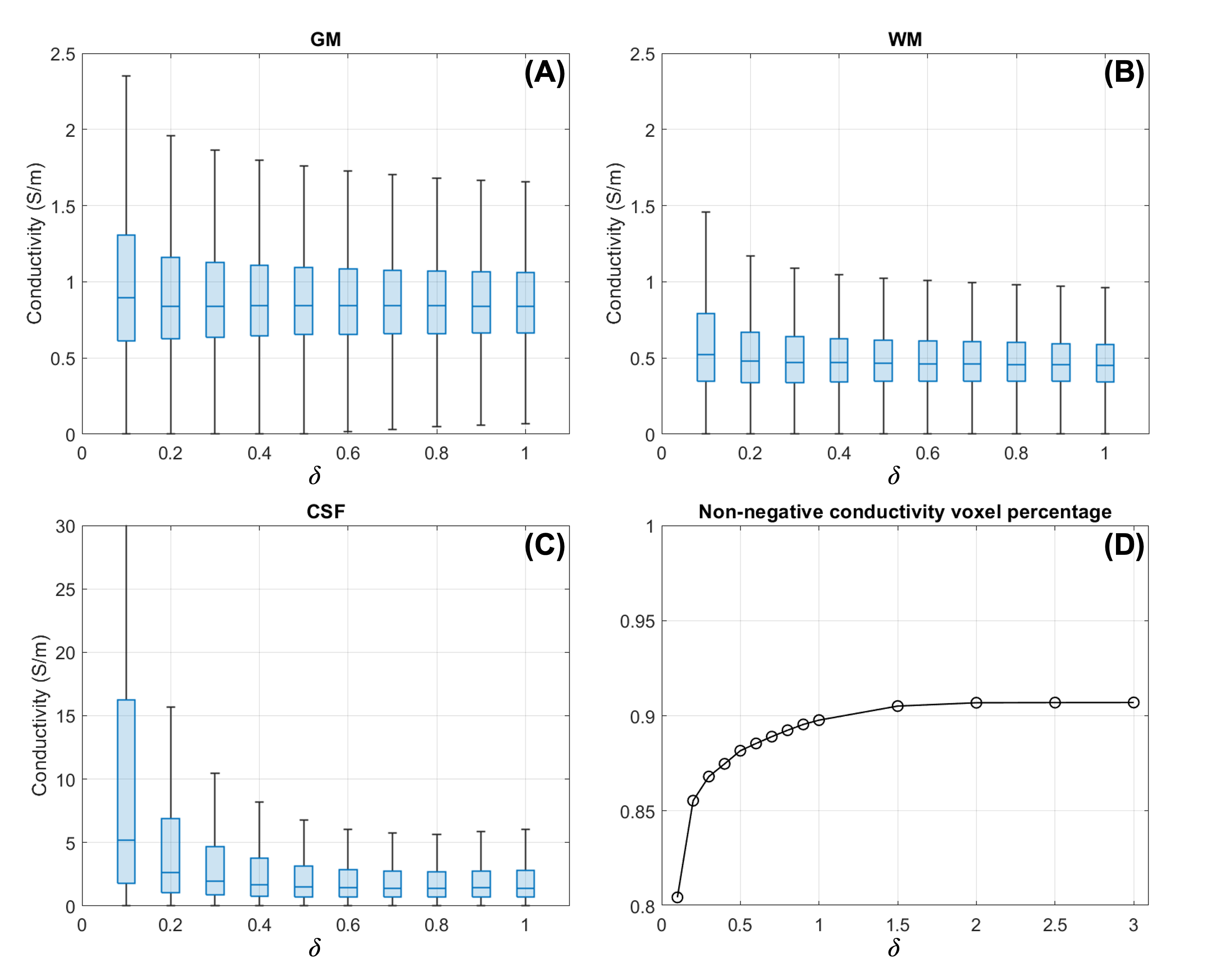
To quantify the impact of $$$\delta$$$, GM, WM and CSF conductivities were measured at different $$$\delta$$$ values, from 0.1 to 3, where $$$W$$$ for each voxel within the kernel became virtually identical. To estimate the reconstruction error, we computed the percentage of brain voxels with non-negative conductivity values.
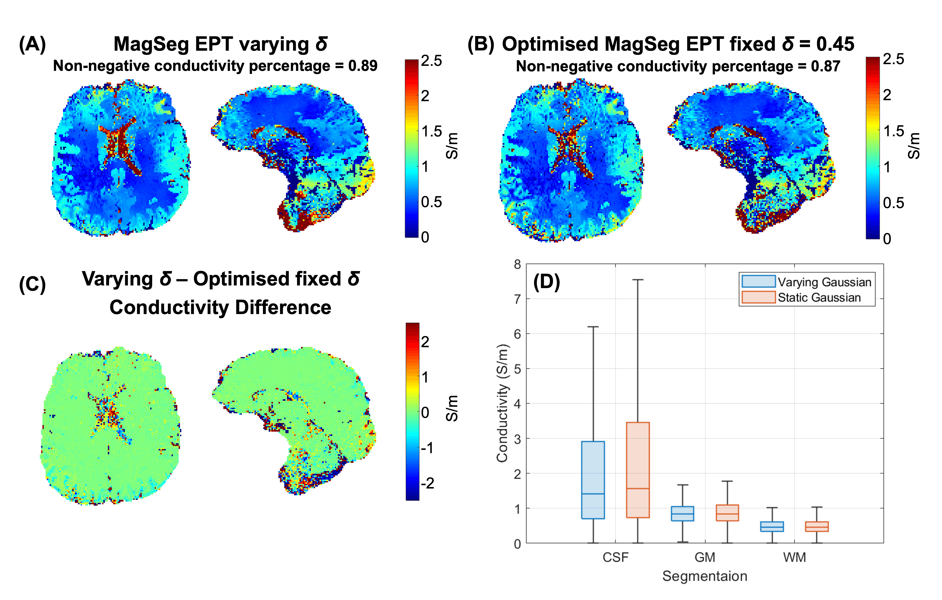
To implement a new magnitude-weighted EPT method that accounts for $$$\phi_{0}$$$ noise levels, $$$\delta$$$ was calculated automatically in each voxel as the inverse, normalized phase noise¹⁴ which was output from the non-linear fit⁹ of the complex data. The results were compared with those obtained with a visually optimised $$$\delta$$$ set to 0.45¹³.

Results and Discussion

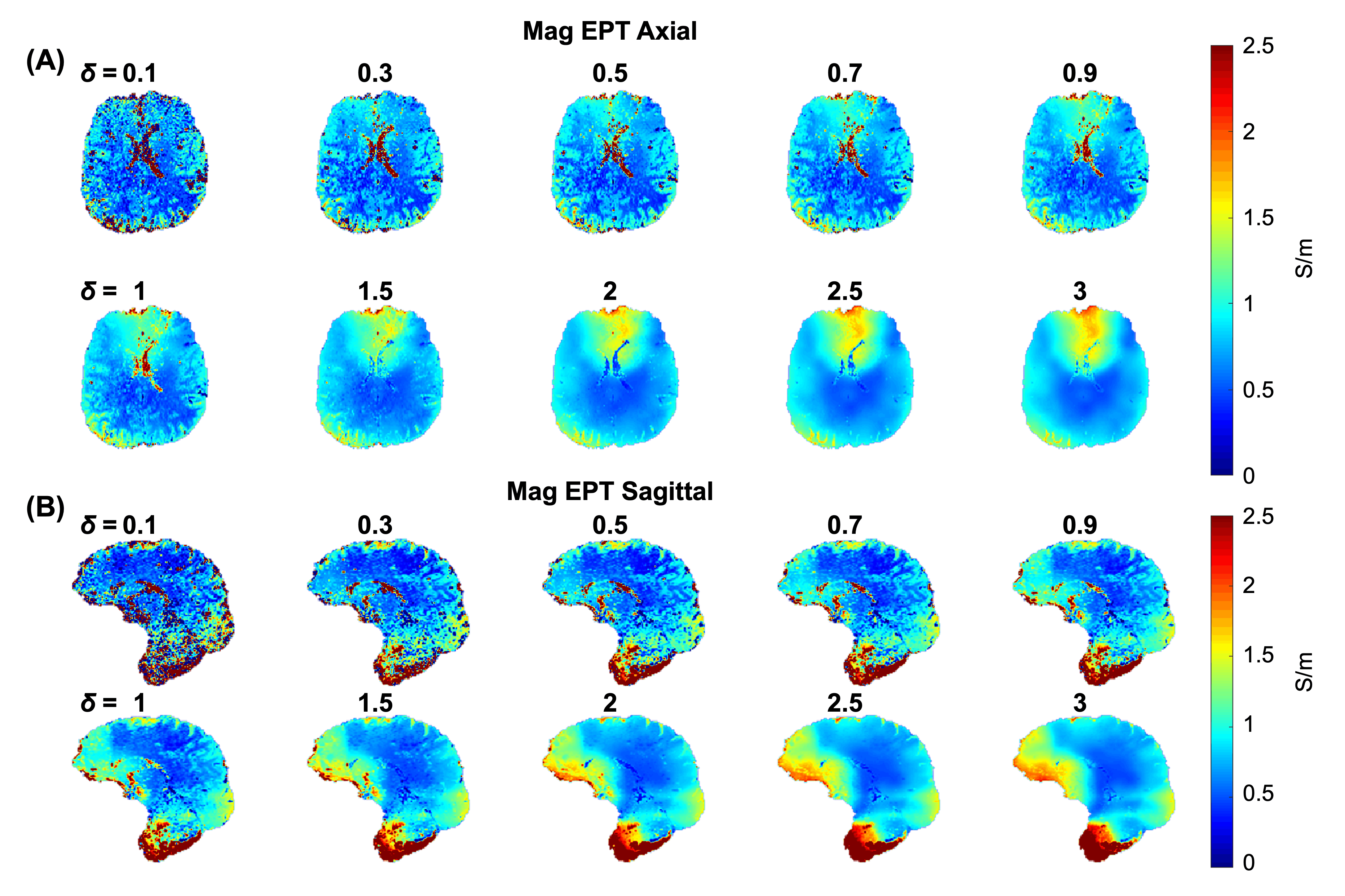
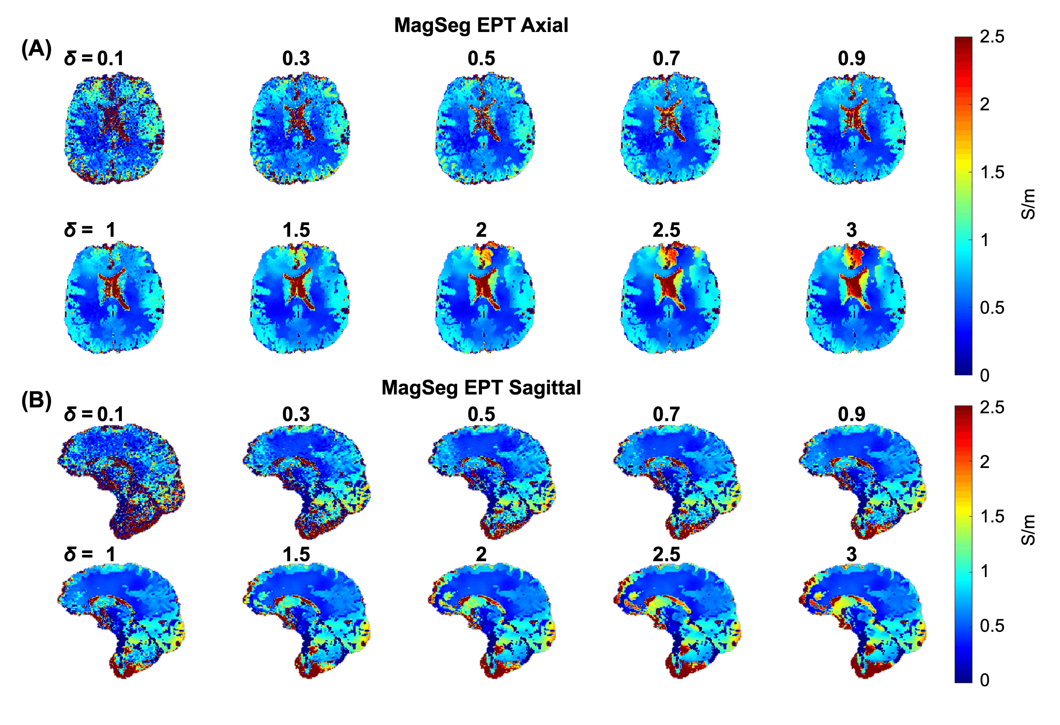
In all conductivity maps, the lower part of the brain contained artifacts due to residual slice-to-slice phase inconsistencies.
For magnitude-weighted EPT (Mag and MagSeg) with fixed $$$\delta$$$, the tissue contrast and noise level of conductivity maps are determined by $$$\delta$$$ (Figures 1 and 3, respectively).
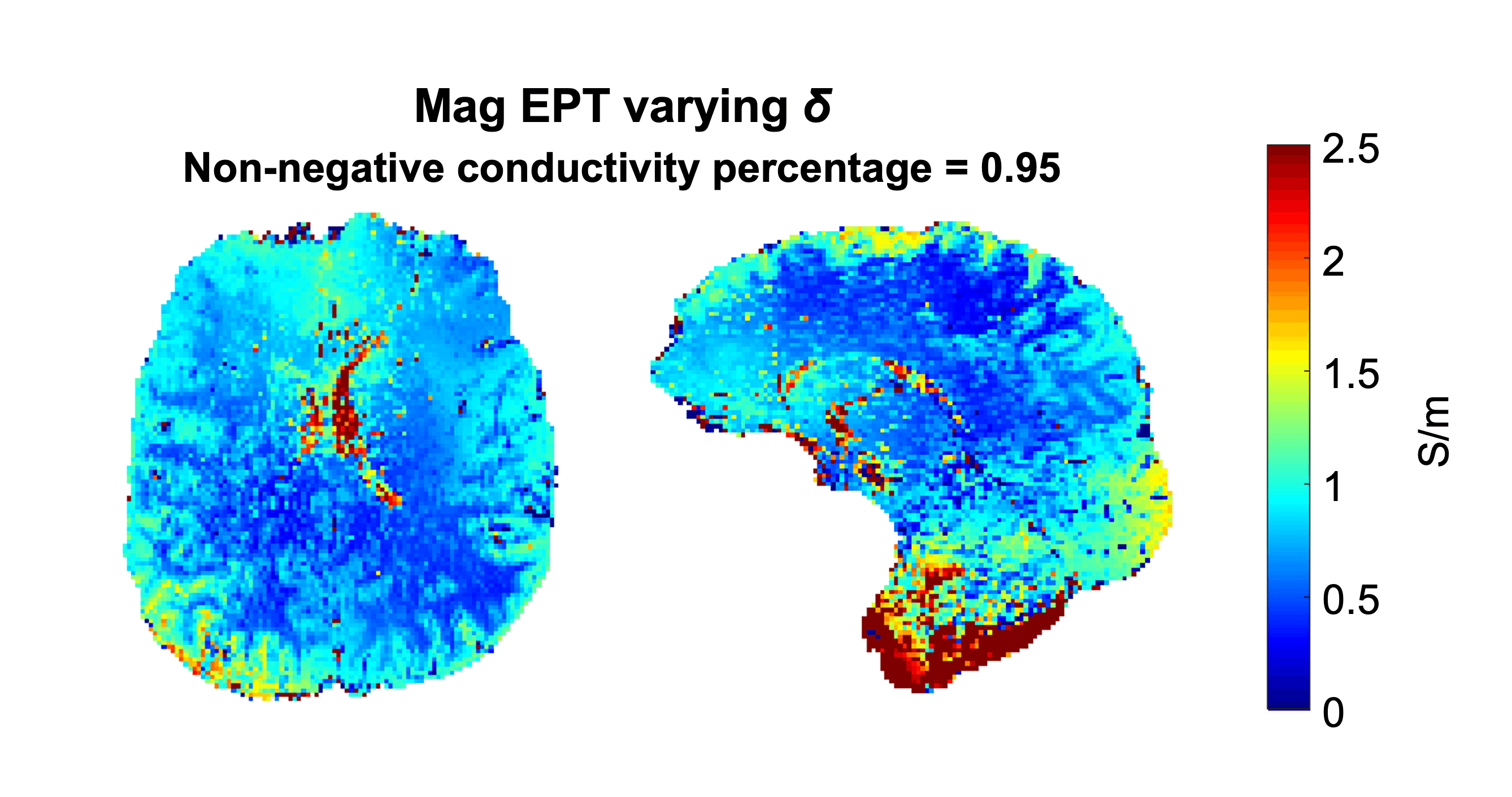
For Mag EPT (Figure 1), the conductivities in GM, WM and CSF varied with $$$\delta$$$ (not shown), while the automatic method with varying $$$\delta$$$ optimised the conductivity map (Figure 2) without tissue segmentations.
For MagSeg EPT (Figure 3), the regional conductivities decreased at different rates with increasing $$$\delta$$$ (Figure 4A-C), while the non-negative conductivity voxel percentage increased with $$$\delta$$$ (Figure 4D).
Compared to the optimised MagSeg conductivity map using fixed $$$\delta$$$, the varying $$$\delta$$$ MagSeg conductivity map showed similar median tissue conductivities, smaller CSF conductivity variation, and fewer voxels with negative conductivities (Figure 5).

Conclusion

We analysed the impact of the standard deviation $$$\delta$$$ of the Gaussian weighting function for magnitude-weighted EPT. $$$\delta$$$ strongly affects the appearance of conductivity maps and tissue conductivity values. We developed a new method to vary $$$\delta$$$ automatically depending on phase noise levels, which generated optimised conductivity maps.

Acknowledgements

The authors are supported by European Research Council Consolidator Grant (DiSCo MRI SFN 770939).

References

[1] U. Katscher, and C. A.T. van den Berg. Electric Properties Tomography: Biochemical, Physical and Technical Background, Evaluation and Clinical Applications, NMR Biomed. 2017; 30(8): e3729.

[2] T. Voigt, et al. Quantitative Conductivity and Permittivity Imaging of The Human Brain Using Electric Properties Tomography. Magn. Reson. Med. 2011; 66(2): 456-466.

[3] S. K. Lee, et al. Theoretical Investigation of Random Noise-Limited Signal-to-Noise Ratio in MR-Based Electrical Properties Tomography, IEEE Trans. Med. Imaging 2015; 34(11): 2220-2232.

[4] A. Karsa, and K. Shmueli. New Approaches for Simultaneous Noise Suppression and Edge Preservation to Achieve Accurate Quantitative Conductivity Mapping in Noisy Images. Proc. Ann. Meeting ISMRM 2021; 3774.

[5] J. Shin, et al, Initial Study on In Vivo Conductivity Mapping of Breast Cancer Using MRI, J. Magn. Reson. Imaging. 2015; 42(2): 371-378.

[6] J. Lee, et al. MR-based Conductivity Imaging Using Multiple Receiver Coils. Magn. Reson. Med. 2016; 76(2): 530–539.

[7] F. Savigny, et al. Robust Reconstruction of Electrical Conductivity Using Anatomically-informed Quadratic Fit. Proc. Ann. Meeting ISMRM 2023; 1626.

[8] U. Katscher et al. Estimation of Breast Tumor Conductivity Using Parabolic Phase Fitting. Proc. Ann. Meeting ISMRM 2012; 3482.

[9] B. Kressler, et al. Nonlinear Regularization for Per Voxel Estimation of Magnetic Susceptibility Distributions from MRI Field Maps. IEEE Trans. Med. Imaging. 2010; 29(2): 273-281.

[10] A. Karsa, and K. Shmueli. SEGUE: A Speedy rEgion-Growing Algorithm for Unwrapping Estimated Phase, IEEE Trans. Med. Imaging. 2018; 38(6): 1347-1357.

[11] O. Arsenov, et al. Rapid In-Vivo Quantitative Conductivity Mapping in the Human Brain Using a Multi-Echo EPI Sequence, Proc. Ann. Conference BIC-ISMRM 2023; PT4-5.

[12] J. Ashburner, et al. SPM12 Manual, Wellcome Trust Centre for Neuroimaging, London. 2021.

[13] A. Karsa, et al., Optimal Kernel Radii for Calculating the Derivatives of Noisy B1 Phase for Accurate Phase-Based Quantitative Conductivity Mapping, Proc. Ann. Meeting ISMRM 2021; 3775.

[14] F. Schweser, et al. Foundations of MRI phase imaging and processing for Quantitative Susceptibility Mapping (QSM). Z. Med. Phys. 2016; 26(1): 6-34.

Figures

Figure 1: Magnitude-weighted Mag conductivity maps with different, fixed δ, shown in (A) axial and (B) sagittal planes. With smaller δ, stronger contrasts were generated between GM, WM and CSF but conductivity maps became noisier. The lower part of the brain suffered from artifacts due to residual slice-to-slice phase inconsistencies.

Figure 2: Magnitude-weighted Mag conductivity map calculated with varying Gaussian width δ. The new automatic method with varying δ optimised the conductivity map, balancing tissue contrast and noise, without tissue segmentations. The lower part of the brain suffered from artifacts due to residual slice-to-slice phase inconsistencies.

Figure 3: Magnitude-weighted MagSeg conductivity maps with different, fixed δ, shown in (A) axial and (B) sagittal planes. Segmentations improve the overall contrast between GM, WM and CSF, but the noise level of conductivity maps is still affected by δ. The pixelwise conductivities were calculated in 3D kernels, determined by local tissue segmentations. The lower part of the brain suffered from artifacts due to residual slice-to-slice phase inconsistencies.

Figure 4: Conductivity values in the MagSeg conductivity maps in Figure 3 within (A) GM, (B) WM and (C) CSF. (D) shows how the percentage of brain voxels with non-negative conductivity values changes with different δ. The regional conductivities decreased at different rates with increasing δ, due to different local noise levels. In contrast, the percentage of brain voxels with non-negative conductivity increased with δ.

Figure 5: MagSeg Conductivity maps with (A) varying Gaussian width δ, (B) fixed Gaussian width δ visually optimised at 0.45, (C) conductivity difference between (A) and (B), showing improvement within ventricles and the cerebellum using varying Gaussian width. (D) Comparison of their non-negative GM, WM and CSF conductivities (outliers not shown). Varying δ MagSeg EPT has median tissue conductivities similar to the optimised fixed δ MagSeg EPT, smaller variation, and fewer negative conductivity voxels.

Proc. Intl. Soc. Mag. Reson. Med. 32 (2024)

3682

DOI: https://doi.org/10.58530/2024/3682