3677
Mobility-weighted Effective Extracellular Ion Concentration Imaging using MRI1Health Systems, Philips Healthcare, Seoul, Korea, Republic of, 2Division of Applied RI, Korea Institute of Radiological and Medical Science, Seoul, Korea, Republic of, 3Department of Hepato-Biliary-Pancreas Surgery, Chonnam National University Medical School, Gwangju, Korea, Republic of, 4Department of Radiology, Chosun University Hospital and Chosun University College of Medicine, Gwangju, Korea, Republic of, 5Biomedical Engineering, Kyung Hee University, Seoul, Korea, Republic of
Synopsis
Keywords: Electromagnetic Tissue Properties, Electromagnetic Tissue Properties, Electrical Conductivity, EPT, Conductivity Tensor Imaging, Metabolite Imaging
Motivation: Extracellular fluid within the brain is complex electrolyte comprising various ions. Disturbances in the balance of electrolytes have been associated with various pathological disorders.
Goal(s): The study aimed to provide quantitative visualization of mobility-weighted effective extracellular ion concentration at every pixel.
Approach: Three phantom experiments were conducted using CTI, precisely controlling ion concentrations, mobilities and cell-alike phantom validation.
Results: The measured values of ion concentrations in three phantoms were comparable to the intended values, demonstrating accuracy. The conductivity tensor imaging method could extract the contribution of ionic concentration and mobility in measured conductivity information.
Impact: We proposed a method to derive the mobility-weighted effective extracellular ion concentration using conductivity tensor imaging (CTI). Ionizing radiation significantly alters the concentration of ions in tissues. Understanding cellular-level ion concentrations is critical for optimizing the effectiveness of radiation therapy.
Introduction
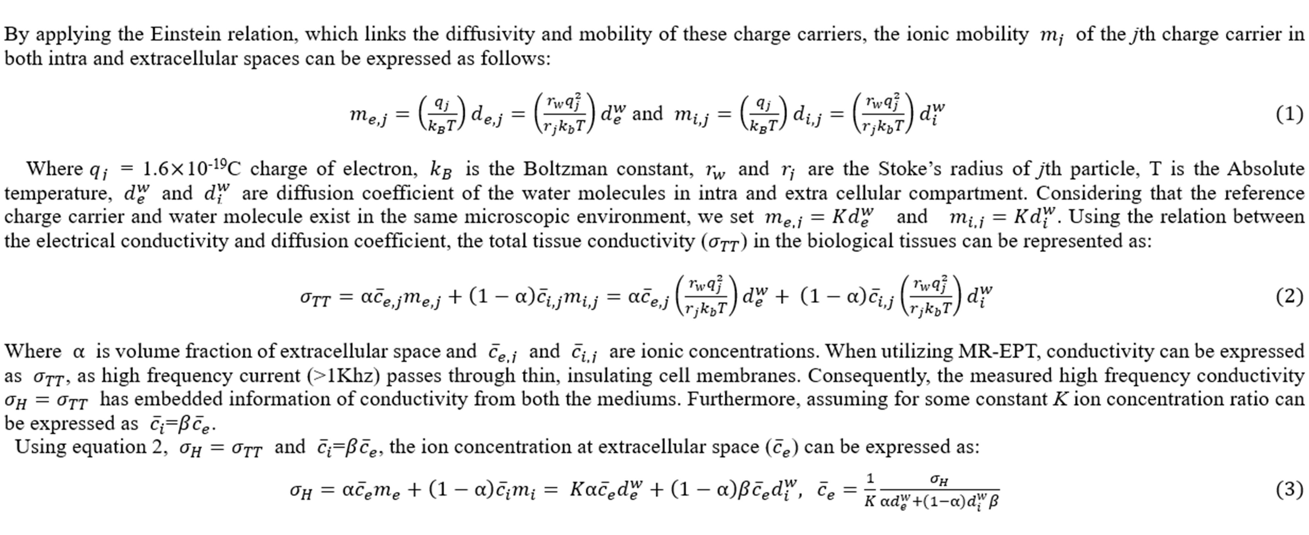
Electrical conductivity of tissues can be decomposed into the ionic concentration and their mobility1. Recently proposed conductivity tensor imaging (CTI) can extrapolate the contrast of ionic concentration from measured high-frequency conductivity from MR-EPT2,3. Fig. 1 explains the reconstruction frame work of mobility-weighted effective extracellular ion concentration (Eq. 3), where $$${\overline{c}_e}$$$ is expressed as:$$\overline{c}_e= \frac{\sigma_H}{\alpha d^w_e + (1-\alpha) d^w_i \beta}$$
Method
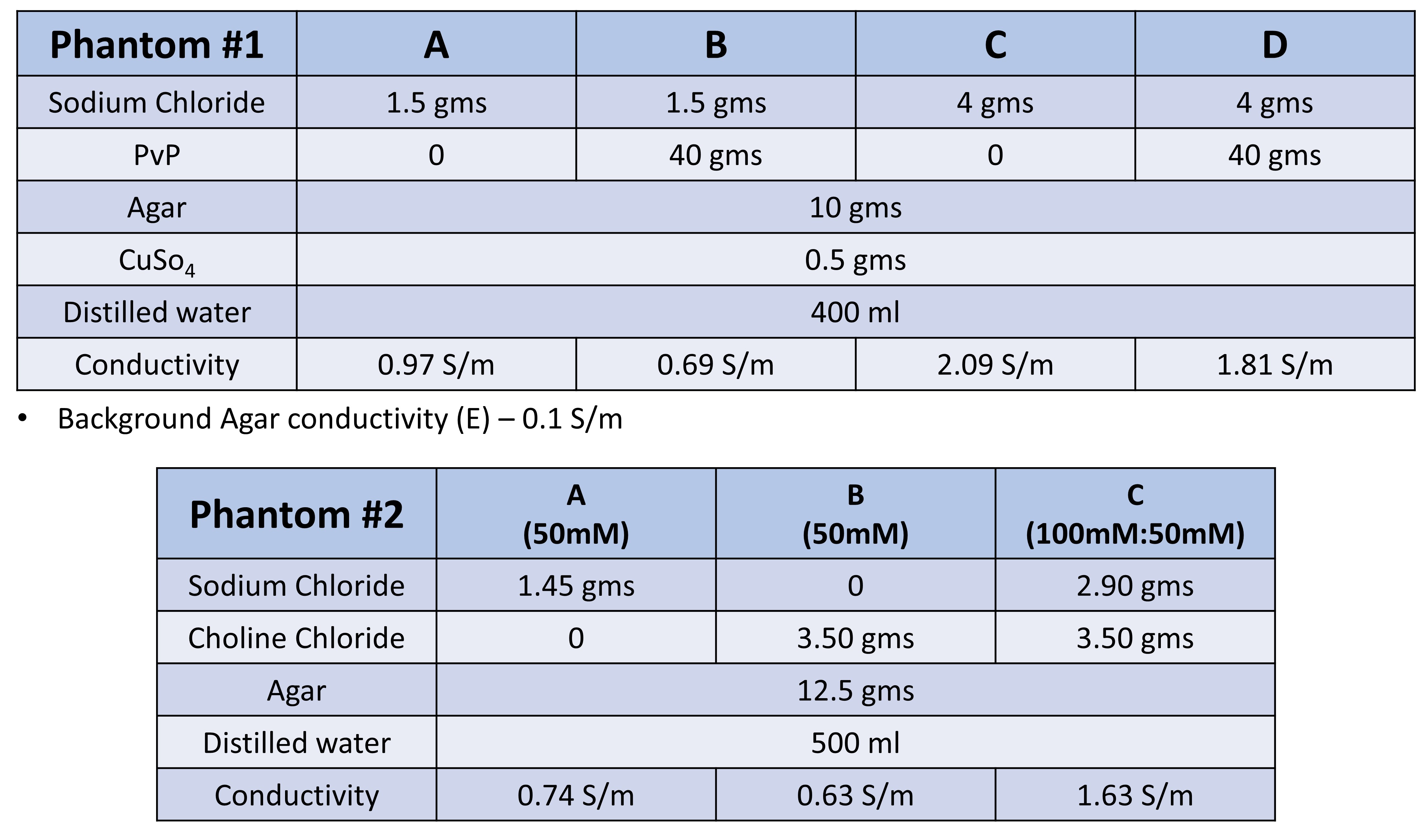
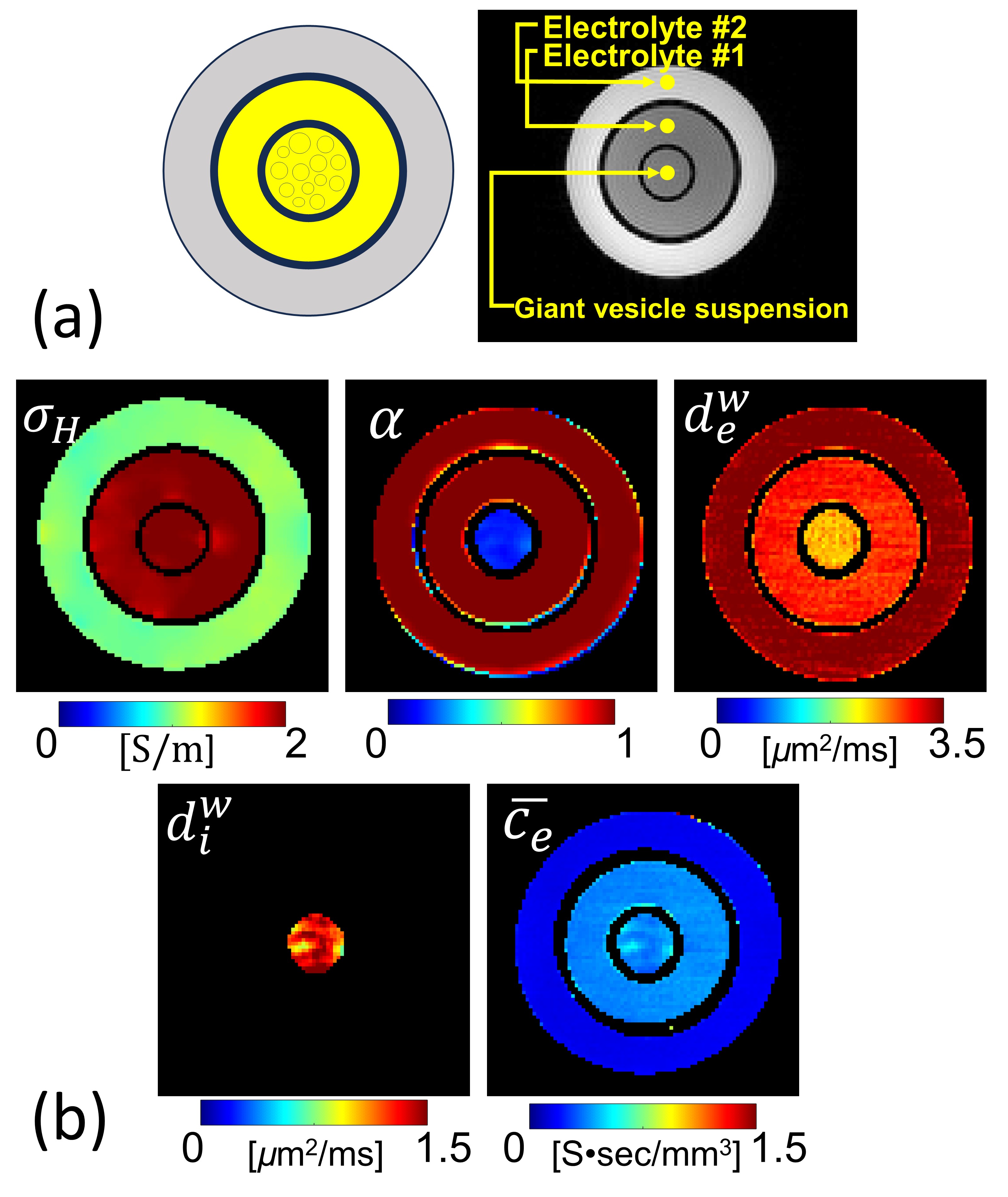
We constructed three experimental phantoms to effectively demonstrate the proposed ion concentration imaging framework. The detailed recipe to build phantom #1 and #2, information of individual anomaly is summarized in Fig. 2. To regulate the mobility of both ions and water molecules, PVP was added only within anomalies B and D in phantom #1. In phantom #2, anomaly C was a mixture of NaCl and choline chloride in a 2:1 ratio. Phantom #3 consists of three compartments, as shown in Fig. 4a. Electrolyte #1 and #2 was 7.5 and 3.5 g/L NaCl. The giant vesicle suspension (GVS) shown in Fig. 2a was filled and suspended with electrolyte #1.CTI experiments were conducted at Kyung Hee University Hospital and KIRAMS, Seoul, using a 3T Achieva TX MRI scanner (Philips Medical Systems, the Netherlands) equipped with an 8-channel head coil, and a 9.4T research MRI scanner (Agilent Technologies, USA) with a single-channel body coil. We employed the multi-echo spin-echo (MSE) imaging sequence to acquire B1 phase maps for reconstructing high-frequency conductivity images of the phantoms. The imaging protocols were as follows: for phantom #1 and #2, TR/TE = 1000/18 ms, Necho=3, flip angle = 90, FOV = 240×240×50 mm3 with spatial resolution of 1.87×1.87×10 mm3. For phantom #3, TR/TE =1500 /15 ms, Necho=6, flip angle = 90, FOV=60×60×2.5 mm3, with an isotropic resolution of 0.5 mm3. A single-shot spin-echo echo-planar (SS-SE-EPI) imaging sequence was used for multi-b-diffusion-weighted imaging. For phantom #1 and #2, the b-values used were 0, 50, 150, 300, 500, 700, 1000, and 1400 s/mm2. For phantom #3, we included additional b-values of 1800, 2200, 2600, 3000, 3500 s/mm2. The number of directions of the diffusion-weighting gradients was 6 for all acquisitions. Reconstruction of CTI parameters is available here1,2.
Results and Discussion
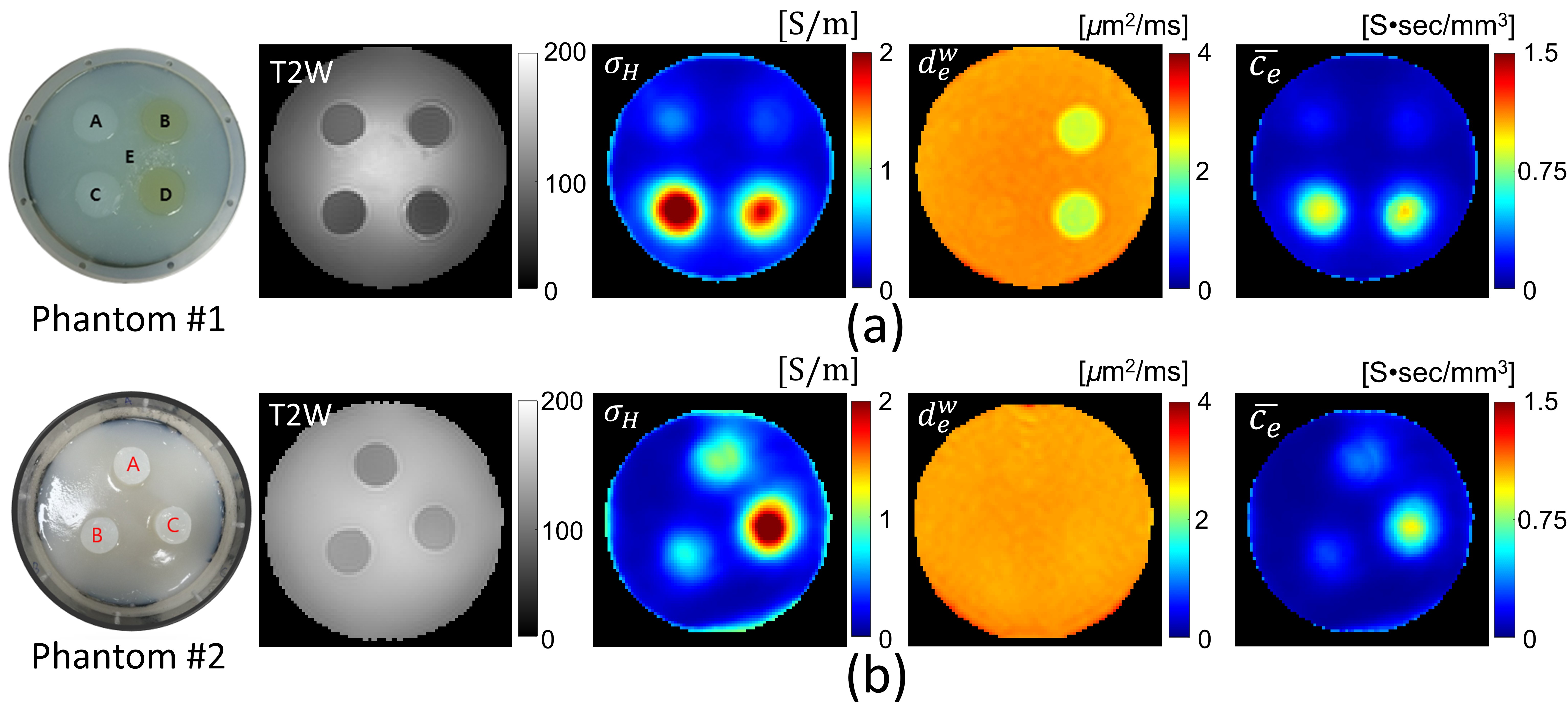
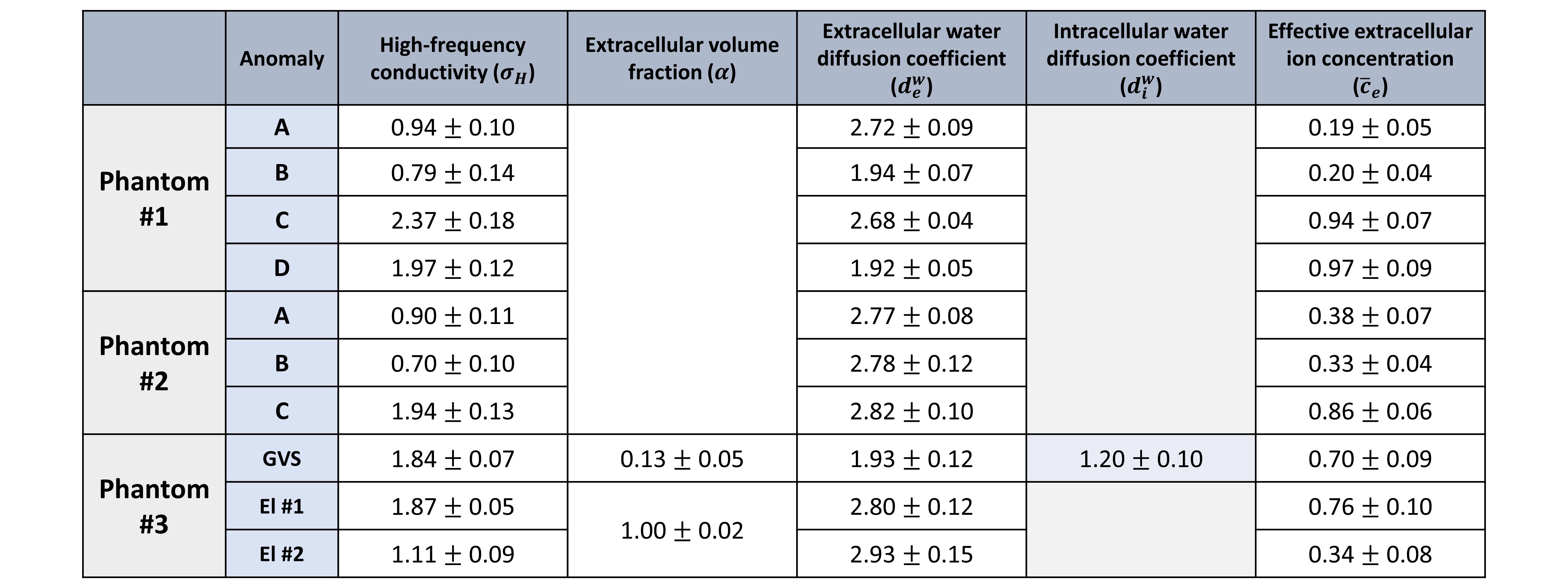
In phantom #1, the ionic concentration was identical in anomalies A and B (also C and D), resulting in a similar contrast in the reconstructed ionic concentration image ($$${\overline{c}_e}$$$) as indicated in Table 3 (Fig. 5). Notably, the mobility of anomalies B and D was observed to be reduced, exhibiting a lower value of diffusion coefficient ($$${d^w_e}$$$).In phantom #2, even though we used similar ionic concentration in anomaly A and B, the measured value (ce) in A was higher by 12%. This discrepancy may have stemmed from the different activity coefficient of NaCl and choline molecules, resulting in higher values. Additionally, in anomaly C, the measured concentration is 2.7 times that of anomaly A, which is consistent with the concentration ratio of ions (2:1) we intended. Fig. 3a and b shows the images of CTI parameters in phantom #1 and #2.
Unlike phantom #1 and #2, we added giant vehicles, creating an intracellular space in phantom #3. In phantom #3, the high-frequency conductivity ($$$\sigma_H$$$) images displayed a higher contrast for Electrolyte #1 and the giant vesicle suspension compared to Electrolyte #2. The contrast rises from the difference in ion concentrations between the two electrolytes. However, when using the same Electrolyte #1 within the giant vesicles, no contrast difference was observed in $$$\sigma_H$$$. The measured values of the parameters in phantom #3 are presented in Table 1. Given the same electrolyte (#1) is used to submerged giant vesicles in inner compartment the measured values of $$${\overline{c}_e}$$$ were found to be similar in both compartments as shown in Fig. 4b and Table 3. We also compared the conductivity values calculated using equation $$$\sigma_L = \alpha \overline{c}_e d_e^w$$$ with impedance analyzer in giant vesicles phantom and observed relative error (%) ranges from 1.1 to 9.2%.
Conclusion
In this study, we employed electrodeless CTI method to visualize the distribution of extracellular ions. Through two separate phantom experiments, where we precisely controlled the concentrations and mobilities of the ions, we validated that the proposed method could extract the ion-concentration information. Moreover, involving the addition of cell alike material we confirmed that measured ion concentration is from extracellular space. The reconstructed parameters vividly explained the effects of ionic concentration and mobility on electrical conductivity. CTI method can be easily implemented in clinical MRI scanners without adding any hardware, promising to augment the precision of radiation therapy and advance treatment outcomes as well as disease ionic microenvironment4.Acknowledgements
The author would like to thank National Research Foundation of Korea (NRF) grants funded by the Korea government (No. 2019R1A2C2088573 and 2021R1A2C2004299).References
- S. Z. K. Sajib et al. Electrodeless conductivity tensor imaging (CTI) using MRI: Basic theory and animal experiments. Biomed. Eng. Lett. 2018;8:273–282.
- Katoch N. et al. Conductivity tensor imaging of in-vivo human brain and experimental validation using giant vesicle suspension. IEEE TMI 38, 1569-1577 (2019).
- Katscher, Ulrich, et al. Magnetic Resonance Electrical Properties Tomography (MREPT). “Electrical Properties of Tissues”. Advances in Experimental Medicine and Biology, 2022, vol. 1380. Springer.
- Park, Ji Ae, et al. In vivo measurement of brain tissue response after irradiation: comparison of T2 relaxation, apparent diffusion coefficient, and electrical conductivity. IEEE Trans. Med.Imaging 2019;38:2779-2784.
Figures