3675
Artifact Reduction for Rapid Phase-Based EPT in the Human Brain In Vivo Using a Multi-Echo 2D EPI Sequence1Medical Physics and Biomedical Engineering, University College London, London, United Kingdom, 2Centre for Medical Image Computing, University College London, London, United Kingdom
Synopsis
Keywords: Electromagnetic Tissue Properties, Image Reconstruction, Electrical Properties Tomography, EPT, Conductivity mapping
Motivation: To date, phase-based electrical properties tomography (EPT) has been performed using time-consuming (~5-minute) gradient-echo sequences.
Goal(s): To calculate EPT conductivity maps from a rapid multi-echo 2D-EPI acquisition (TR~4s), overcoming slice-to-slice phase inconsistencies.
Approach: We investigated the effect of four different methods to remove slice-to-slice inconsistencies from the phase offset (φ0) of the multi-echo 2D-EPI data on conductivity maps in a numerical phantom and in vivo.
Results: Removing the median φ0 in each slice in the brain provided high quality conductivity maps with clear delineation between grey matter, white matter and CSF. Tissue conductivity values showed good inter- and intra-subject repeatability
Impact: We developed a rapid, repeatable method for phase-based EPT from multi-echo 2D-EPI, overcoming slice-to-slice phase inconsistencies. This will facilitate clinical applications of EPT, particularly in studies already using multi-echo 2D-EPI for fMRI, and paves the way towards functional EPT.
Introduction
Phase-based EPT has potential clinical applications1-4 but is performed using time-consuming spin-echo1-3 or gradient-echo4 sequences. Multiple-echo 2D echo-planar imaging (ME-2D-EPI) could allow rapid EPT. However, the phase of 2D-EPI data suffers from slice-to-slice inconsistencies that affect EPT conductivity maps. We tested four methods to remove these in a numerical phantom and in vivo. The intra- and inter-subject repeatability of EPT was then investigated in two healthy volunteers.Methods
DataWe acquired ME5 2D-EPI brain images in two healthy volunteers on a 3T Siemens Prisma with 1.3 mm isotropic resolution, matrix size=184x168x126, BW= 1812 Hz/Pixel, FA=90°, 3 TEs, TE=14.80/39.33/63.86 ms and TR=4034 ms, with multiband 3 and GRAPPA 4 for 70 repeated volumes. Both volunteers were scanned twice, one with a 32-channel head coil (acquisitions 1 and 2) and the other with a 64-channel head coil (acquisitions 3 and 4).
A reference ME 3D-GRE image of the first volunteer was acquired with 1 mm isotropic resolution, matrix size=192x256x176, BW=280 Hz/Pixel, FA=15°, 5 TEs, TE1/ΔTE/TE4 =4.92/4.92/24.60 ms, TR=30 ms, and R=4 and processed with the same EPT pipeline.
A numerical phantom with 1 mm isotropic resolution, realistic conductivity values (σ) and φ0 simulated at 3T6 with noise added to match the EPI SNR was used to evaluate four artifact correction methods. Random slice offsets with similar values as observed in vivo were added to φ0.
EPT
The phase offset at TE=0, φ0, was extrapolated from a non-linear fit7 of the complex data over all echoes for each timepoint and unwrapped8. A mask was generated using FSL BET9, refined by thresholding10,11, and eroded by 1 voxel. Conductivity maps were calculated from masked φ0 maps, using the integral form of the truncated Helmholtz equation12, with magnitude-weighted second-order polynomial fitting13,14. Large 3D spherical kernels (differentiation kernel: 17 voxels, surface integral kernel: 47 voxels) refined using the local tissue segmentation of gray matter (GM), white matter (WM), and cerebrospinal fluid (CSF)14-16 were used to reduce noise and preserve anatomy. The echo-combined magnitude17 was used for magnitude-weighting segmentation with SPM1218-19.
Artifact correction methods
Aiming to remove slice-to-slice inconsistencies in the masked, unwrapped EPI φ0, we subtracted the 1) mean φ0 in each axial slice, 2) median φ0 in each axial slice, 3) φ0 in voxels along a line from each axial slice or 4) used 2D derivative and integral kernels20.
To compare the effect of these four correction methods in the phantom, the root mean square error (RMSE) between σ for each method, Figure 1II.c-f, and the ground truth conductivity (reconstructed from the simulated φ0), Figure 1II.a, was calculated.
Results and Discussion
The lowest RMSE was obtained using mean (44.4%) and median (43.8%). σ in CSF, GM, and WM for mean and median were similar to the ground truth (Figure 2). The line is affected by the noise, overestimating σ and having a larger spread. For the phantom, σ using 2D kernels had smaller variations and were closer to the true values.In vivo, mean and median corrections created smoother φ0 than line, Figure 3I.c-e, which resulted in better tissue contrast in the σ maps, Figure 3II.c-e. In-vivo, using 2D kernels greatly reduced contrast and underestimated CSF σ, Figure 3II.f and Figure 4A. After all four corrections, the bottom of the brain contained artifacts due to residual slice-to-slice inconsistencies. σ using line correction contains large variations in CSF, Figure 4. In GM and WM, mean and median have similar distributions, but in CSF, median mean σ was closer to the GRE reference.
Therefore, we used the median correction method for acquisitions 1-4. Taking the median in each voxel of non-negative conductivities of all co-registered reconstructions over time provided high quality conductivity maps with high contrast and low noise (Figure 5A) except for residual artifacts at the brain’s base. Temporal variations in mean σ were higher in CSF than in GM and WM (Figure 5B), perhaps due to CSF pulsation22. σ showed good intra- and inter-subject repeatability , (Figure 5C), in GM and WM, with more variability in CSF. To quantify the repeatability, the minimum detectable effect (MDE)10,23 was calculated for all ROIs (Figure 5D). WM has the highest intra and inter-subject repeatability (lowest MDEs).
Conclusions
We developed a simple method to remove slice-to-slice inconsistencies in 2D-EPI φ0 maps, based on subtracting the median in each axial slice, which provided the most accurate brain conductivity maps that had good repeatability within and across subjects. Combining conductivity maps across 70 timepoints greatly reduced noise.Acknowledgements
OA, JL, AK, PF and KS are supported by European Research Council Consolidator Grant DiSCo MRI SFN 770939. OK was supported by EPSRC Doctoral Training Partnership (EP/R513143/1).References
1. Shin J, Kim MJ, Lee J, Nam Y, Kim MO, Choi N, Kim S, Kim DH. Initial study on in vivo conductivity mapping of breast cancer using MRI. Journal of Magnetic Resonance Imaging. 2015 Aug;42(2):371-8.
2. Tha KK, Katscher U, Yamaguchi S, Stehning C, Terasaka S, Fujima N, Kudo K, Kazumata K, Yamamoto T, Van Cauteren M, Shirato H. Noninvasive electrical conductivity measurement by MRI: a test of its validity and the electrical conductivity characteristics of glioma. European radiology. 2018 Jan;28:348-55.
3. Park S, Jung SM, Lee MB, Rhee HY, Ryu CW, Cho AR, Kwon OI, Jahng GH. Application of High-Frequency Conductivity Map Using MRI to Evaluate It in the Brain of Alzheimer's Disease Patients. Frontiers in Neurology. 2022 May 16;13:872878.
4. Wang Y. Magnetic Resonance based Electrical Properties Tomography (EPT) Using Multi-channel Transmission for Imaging Human Brain and Animal Cancer Models (Doctoral dissertation, University of Minnesota). 2018.
5. CMRR. Multi-Band Accelerated EPI Pulse Sequences. https://www.cmrr.umn.edu/multiband/. 2022.
6. Meerbothe TG, Meliado EF, Stijnman PR, van den Berg CA, Mandija S. A database for MR‐based electrical properties tomography with in silico brain data—ADEPT. Magnetic Resonance in Medicine. 2023.
7. Liu T, Wisnieff C, Lou M, Chen W, Spincemaille P, Wang Y. Nonlinear formulation of the magnetic field to source relationship for robust quantitative susceptibility mapping. Magnetic resonance in medicine. 2013 Feb;69(2):467-76.
8. Karsa A, Shmueli K. SEGUE: A speedy region-growing algorithm for unwrapping estimated phase. IEEE Transactions on Medical Imaging. 2018 Dec 11;38(6):1347-57.
9. Smith SM. Fast robust automated brain extraction. Human brain mapping. 2002 Nov;17(3):143-55.
10. Karsa A, Punwani S, Shmueli K. An optimized and highly repeatable MRI acquisition and processing pipeline for quantitative susceptibility mapping in the head‐and‐neck region. Magnetic Resonance in Medicine. 2020 Dec;84(6):3206-22.
11. Kiersnowski OC, Shmueli K. A Novel Gradient-Based Thresholding Method to Improve Brain Masking for Quantitative Susceptibility Mapping. In: British & Irish Chapter of the ISMRM Post-Graduate Symposium. 2023.
12. Voigt T, Katscher U, Doessel O. Quantitative conductivity and permittivity imaging of the human brain using electric properties tomography. Magnetic Resonance in Medicine. 2011 Aug;66(2):456-66.
13. Lee J, Shin J, Kim DH. MR‐based conductivity imaging using multiple receiver coils. Magnetic resonance in medicine. 2016 Aug;76(2):530-9.
14. Karsa A, Shmueli K. New Approaches for Simultaneous Noise Suppression and Edge Preservation to Achieve Accurate Quantitative Conductivity Mapping in Noisy Images. In: Proceedings of ISMRM & SMRT Annual Meeting. 2021.
15. Katscher U, Djamshidi K, Voigt T, Ivancevic M, Abe H, Newstead G, Keupp J. Estimation of breast tumor conductivity using parabolic phase fitting. In: Proceedings of the 20th Annual Meeting of ISMRM, Melbourne, Australia 2012 May 5 (p. 3482).
16. Huang L, Schweser F, Herrmann KH, Krämer M, Deistung A, Reichenbach JR. A Monte Carlo method for overcoming the edge artifacts in MRI-based electrical conductivity mapping. In: Proceedings of 22th Annual Meeting ISMRM 2014 (Vol. 3190).
17. Poser BA, Norris DG. Investigating the benefits of multi-echo EPI for fMRI at 7 T. Neuroimage. 2009 May 1;45(4):1162-72.
18. Ashburner J. SPM: a history. Neuroimage. 2012 Aug 15;62(2):791-800.
19. Friston KJ, Holmes AP, Worsley KJ, Poline JP, Frith CD, Frackowiak RS. Statistical parametric maps in functional imaging: a general linear approach. Human brain mapping. 1994;2(4):189-210.
20. Mandija S, Petrov PI, Vink JJ, Neggers SF, van den Berg CA. Brain tissue conductivity measurements with MR-electrical properties tomography: an in vivo study. Brain topography. 2021 Jan;34:56-63.
21. Gabriel S, Lau RW, Gabriel C. The dielectric properties of biological tissues: III. Parametric models for the dielectric spectrum of tissues. Physics in medicine & biology. 1996 Nov 1;41(11):2271.
22. Katscher U, Stehning C, Tha KK. The impact of CSF pulsation on reconstructed brain conductivity. InProceedings of the 26th science meeting international society for magnetic resonance in medicine Paris, France 2018 (Vol. 546).
23. Bloom HS. Minimum detectable effects: A simple way to report the statistical power of experimental designs. Evaluation review. 1995 Oct;19(5):547-56.
Figures
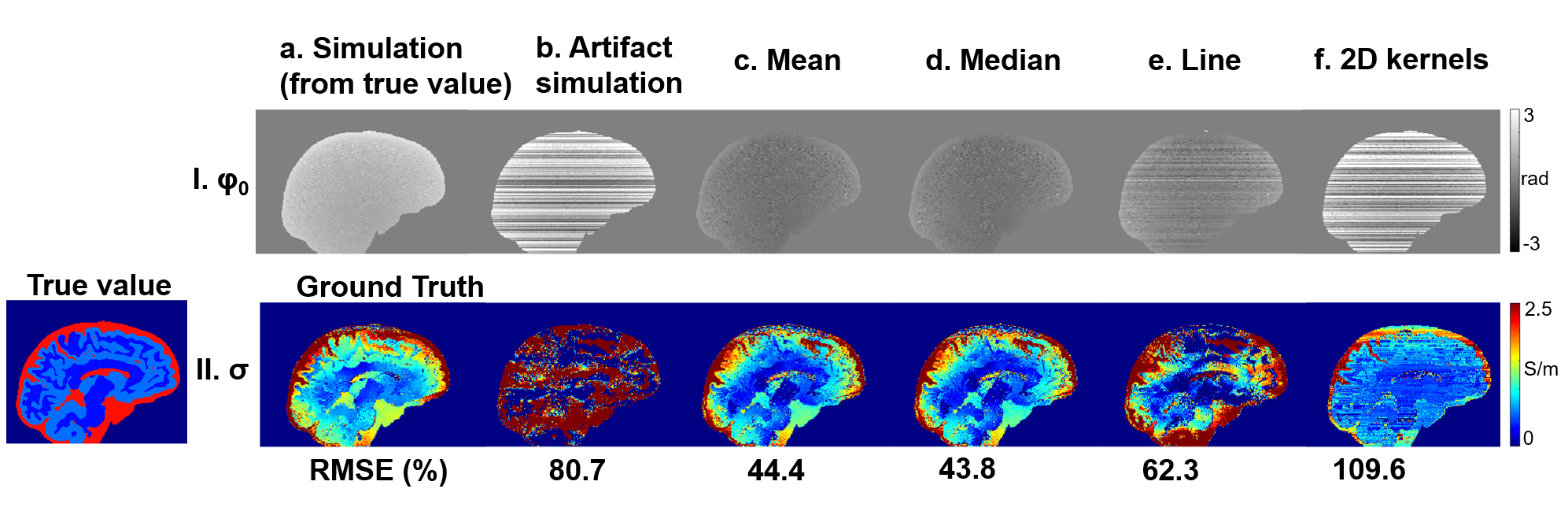
Figure 1. φ0 (I) and conductivity maps (II) for the numerical phantom. Slice-to-slice inconsistencies were added (I.b) to the φ0 simulated (I.a) from the true conductivity values (bottom left). Four correction methods (subtracting the mean, median, line and using 2D kernels) results on φ0, (I.c-f), with corresponding s (II.a-f). The RMSE between the s for each correction and the ground truth, II.a, calculated from the simulated φ0 (I.a) are displayed under each method.
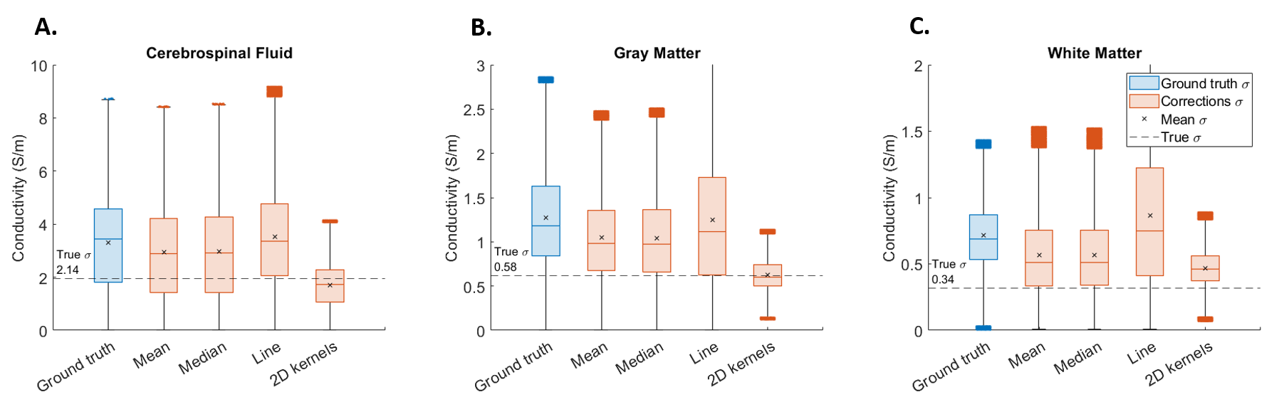
Figure 2. Conductivity distributions in three regions of interest (A: CSF, B: GM, and C: WM), for the numerical phantom. The results for the four correction methods (orange) are compared to the ground truth (blue) in each region. The line in each box is the median conductivity and the cross shows the mean conductivity. The true phantom conductivity values are shown as a black dashed line. Only non-negative conductivity values were included in these distributions.
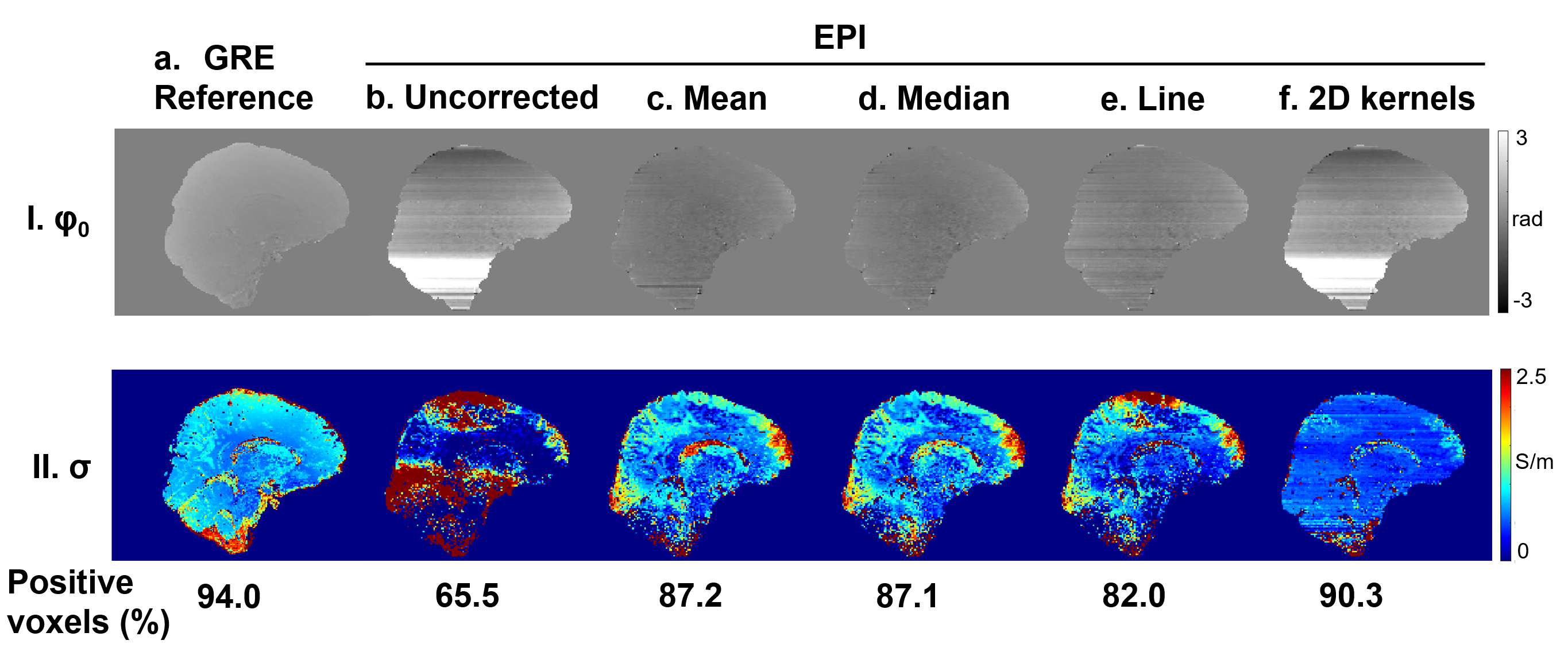
Figure 3. φ0 (I) and conductivity maps (II) in vivo for the GRE reference scan (a) and uncorrected EPI scan (b) compared to EPI corrected with the four different methods (c-f). For the EPI scan the maps correspond to acquisition 1, 6th timepoint. The percentages of voxels in the brain with positive conductivity values are displayed under each map.
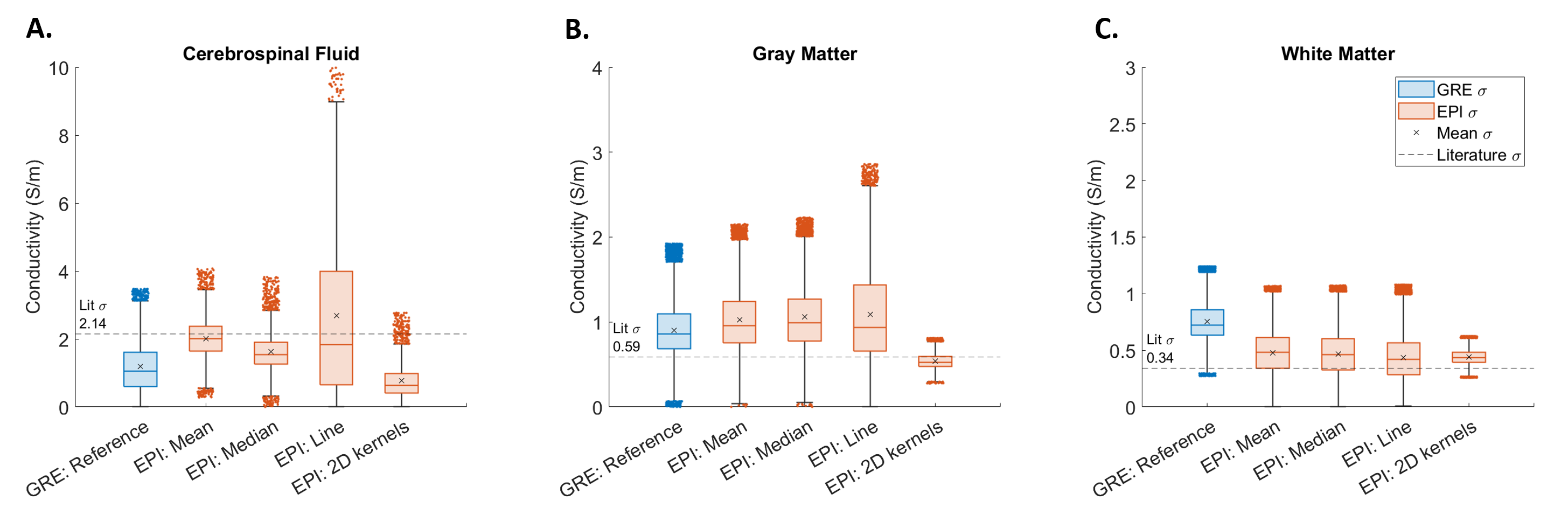
Figure 4. Conductivity distributions in three regions (A:CSF, B:GM, and C:WM) for the reference 3D-GRE (blue) and the 2D-EPI with the four correction methods (orange) shown in Figure 3. The line in each box is the median conductivity and the cross shows the mean conductivity. Literature values measured ex vivo21, are shown as a black, dashed line. Only non-negative conductivity values were included in these distributions.
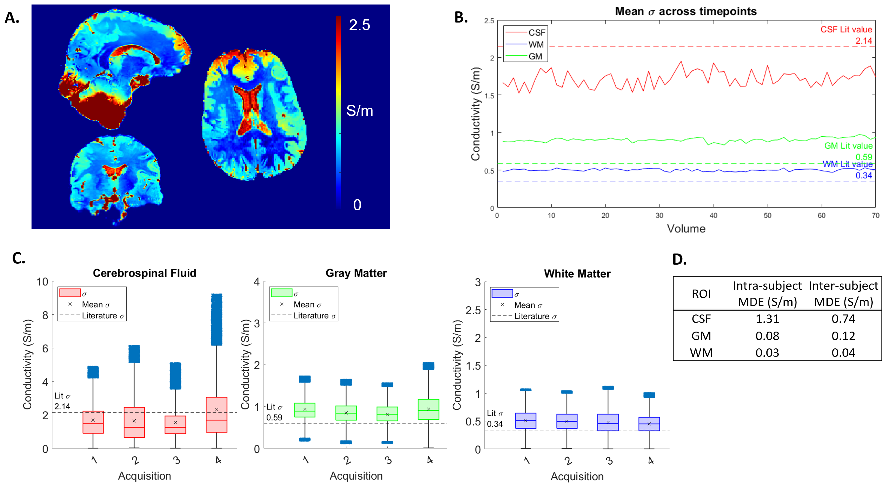
Figure 5. (A) Conductivity map from acquisition 1 calculated as the median of s≥0 over all 70 co-registered timepoints φ0 maps for each timepoint were corrected using the median method. Mean positive s values in CSF, GM, and WM over time for acquisition 1 (B). ROI s distributions of the median EPT across timepoints for volunteer 1: acquisitions 1 and 2; volunteer 2: acquisitions 3 and 4) (C). Minimum detectable effect sizes (MDEs) for each ROI (D).