Recent studies report that line-scan MRI imaging sequences^1-4 can record thalamic and cortical neural electrical responses to stimuli in mice⁵ and humans⁶. The MRI time series appear to match electrophysiological measurements at millisecond resolution. However, other groups following similar protocols have been unable to replicate these results^7-9.
The line-scan acquisition protocol is unlike most functional measurements. Each k-space line is acquired repeatedly at very high (millisecond) temporal resolution. The complete set of lines needed to create a single image is acquired over an extended period of time (tens of seconds). The noise characteristics of this acquisition, particularly of a brain substrate that varies over time, may pose specific challenges in detecting a neural signal. Here we quantify the spatial and temporal properties of the noise in a line-scan acquisition measured from the human brain using a 3T MRI scanner.
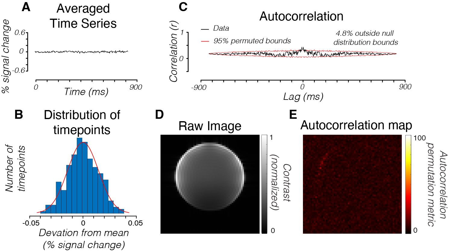
First, we acquired line-scan data from a slice of an agar phantom (Fig 1A). To quantify the temporal structure of the noise, we computed the autocorrelation of the time series. We then compared the amplitude of this autocorrelation with the expected amplitude when the time series is randomly shuffled, removing any temporal structure. The fraction of time points at which the autocorrelation amplitude exceeds the shuffled autocorrelation amplitude is reported as the autocorrelation permutation metric (APM). This metric quantifies the temporal structure in the time series. We observed only a small deviation from unstructured Gaussian noise in the phantom averaged across all voxels in the phantom (Fig 1C). Individual voxels in the phantom also had low APMs (Fig 1E).
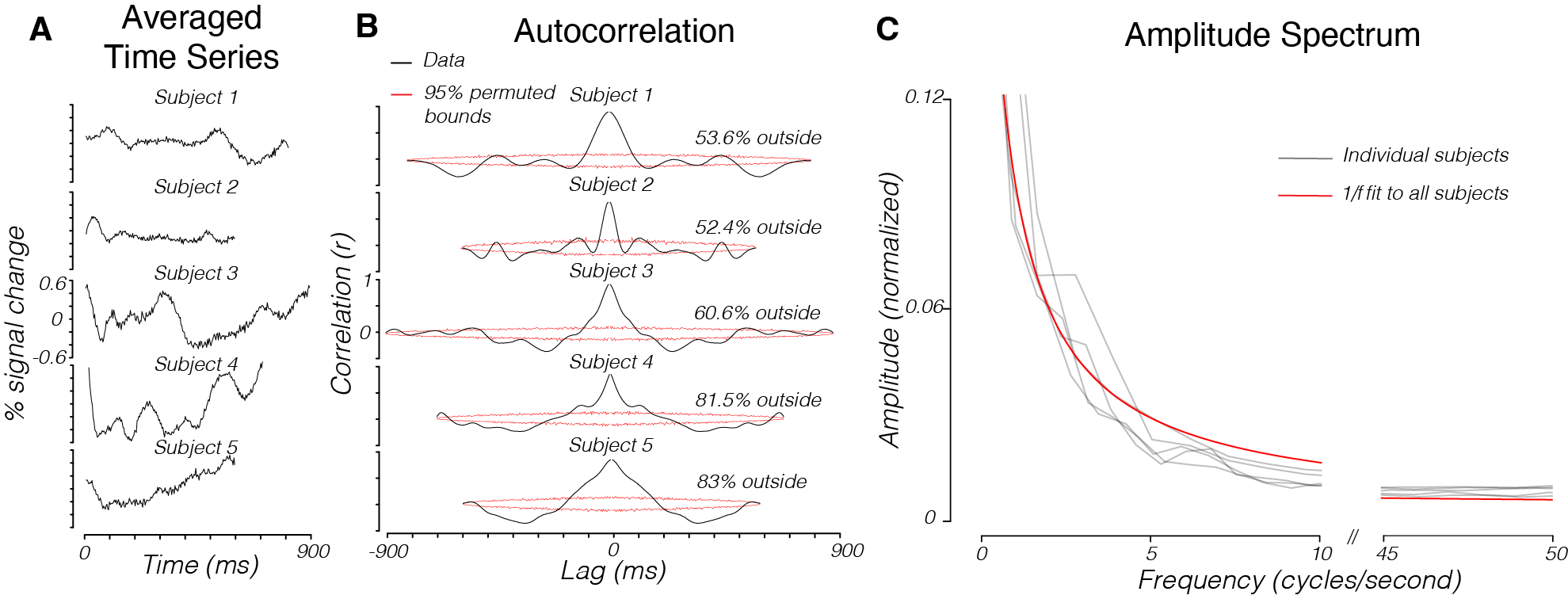
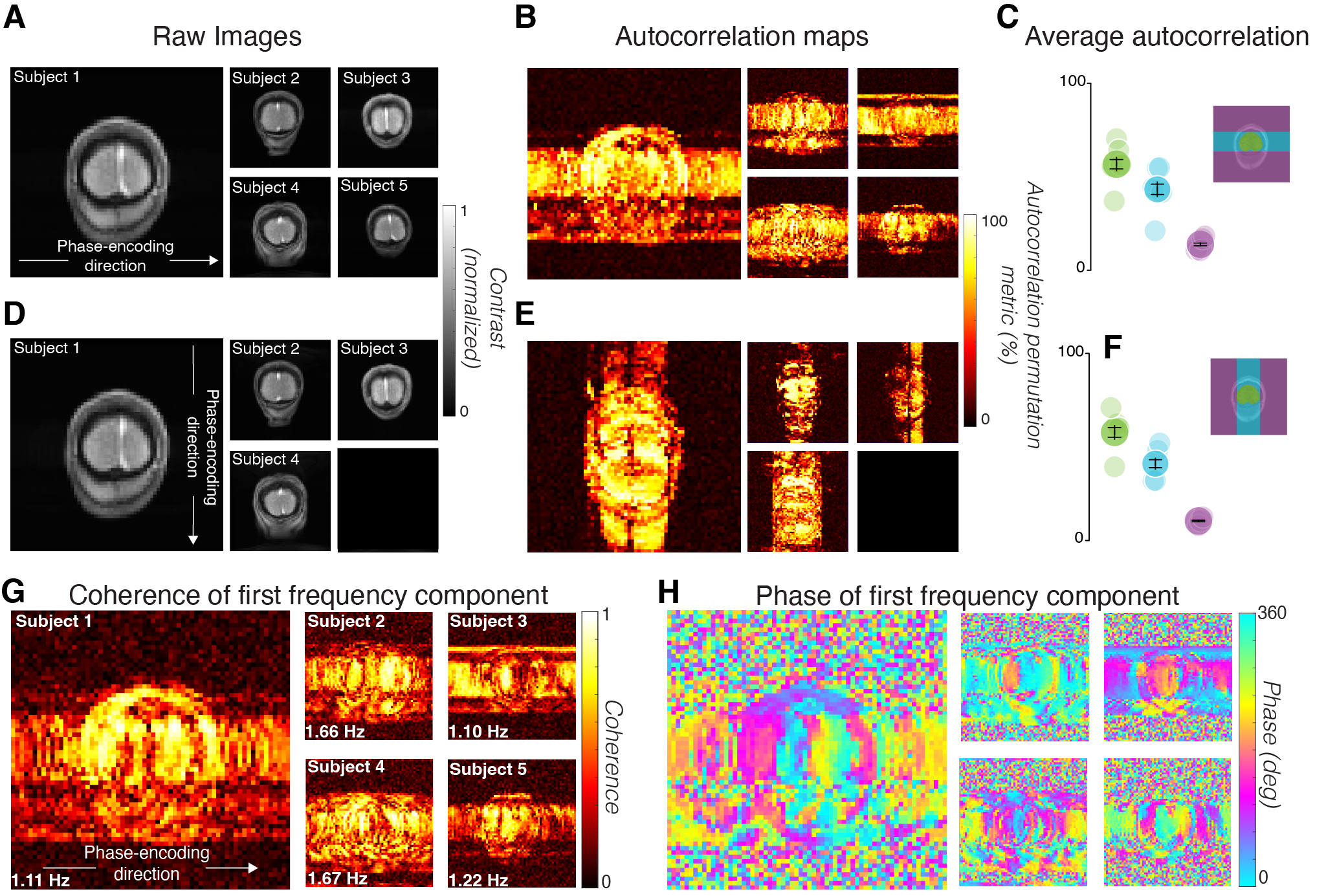
We then collected line-scan data with similar parameters from slices of human brain that included early visual cortex (V1-V3) while subjects viewed a blank screen. Unlike measurements from the phantom, the human brain time series had substantial temporal structure (Fig 2A), as evidenced by high APM values (Fig 2B). Samples from the noise time series are quite similar to expected responses to brief visual stimuli. The temporal structure is apparent when averaging the time series across voxels. The temporal structure is also evident in individual voxels in the brain (figure 3B,E). These modulations have a 1/f dropoff in amplitude (Fig 2C).
Voxels with high APM values were found in the brain, in the skull, and in the empty volume outside the head. Many voxels that contained a segment of the brain within its phase-encoding line had high APM values, even outside of the head (Fig 3B). The spread is always along the phase-encoding direction (compare scans with different phase-encoding directions, Figs 3B, 3E).
Measures of the fundamental temporal frequency component in the response reveal the spatial spread of the signal. Like the APM, the amplitude of the fundamental frequency is high across the head and spreads along the phase-encoding direction (Fig 3G). The phase of the fundamental component varies smoothly along the phase-encoding direction from the brain, and is nearly constant along the perpendicular direction, revealing systematic timing variations (Fig 3H).
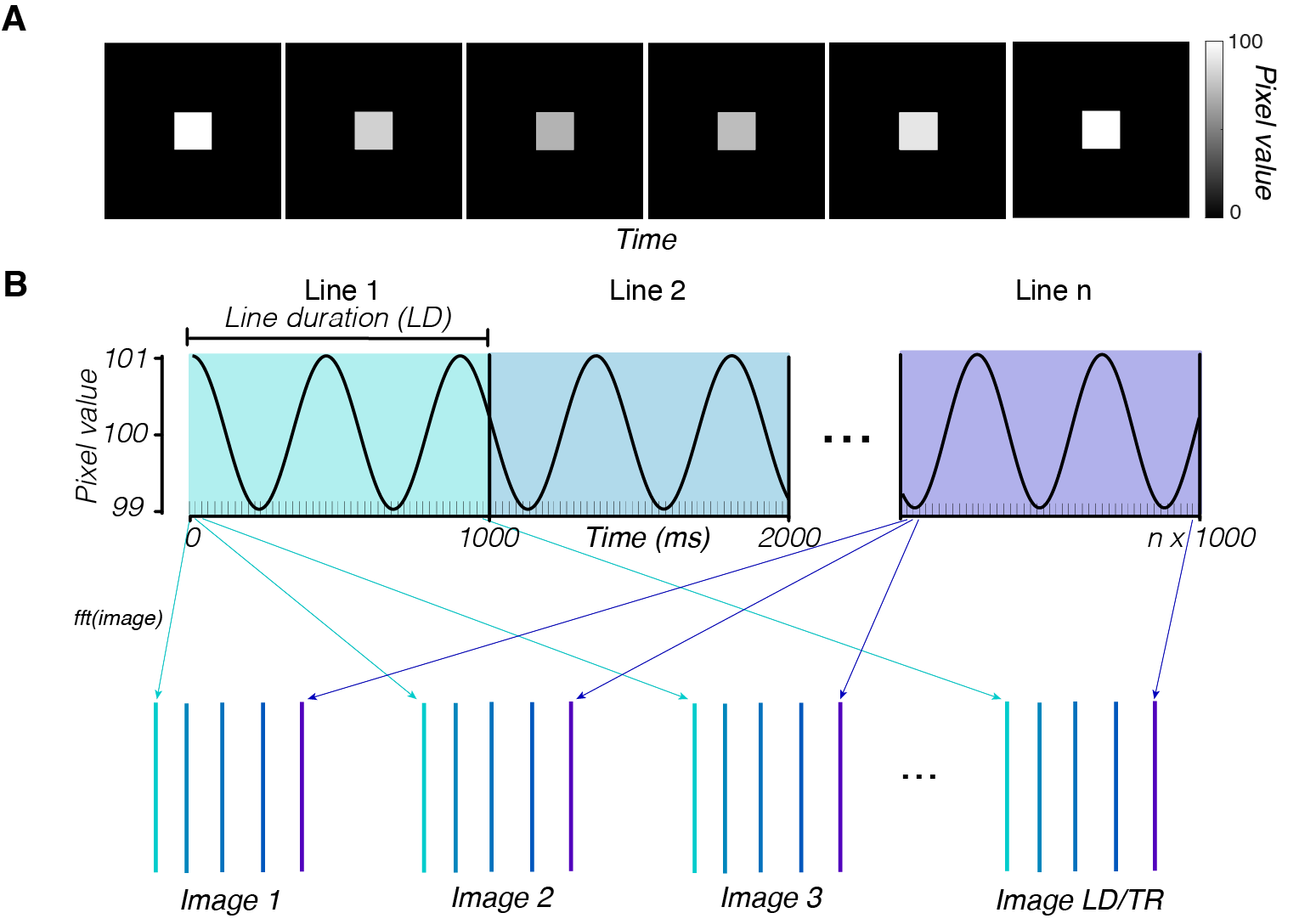
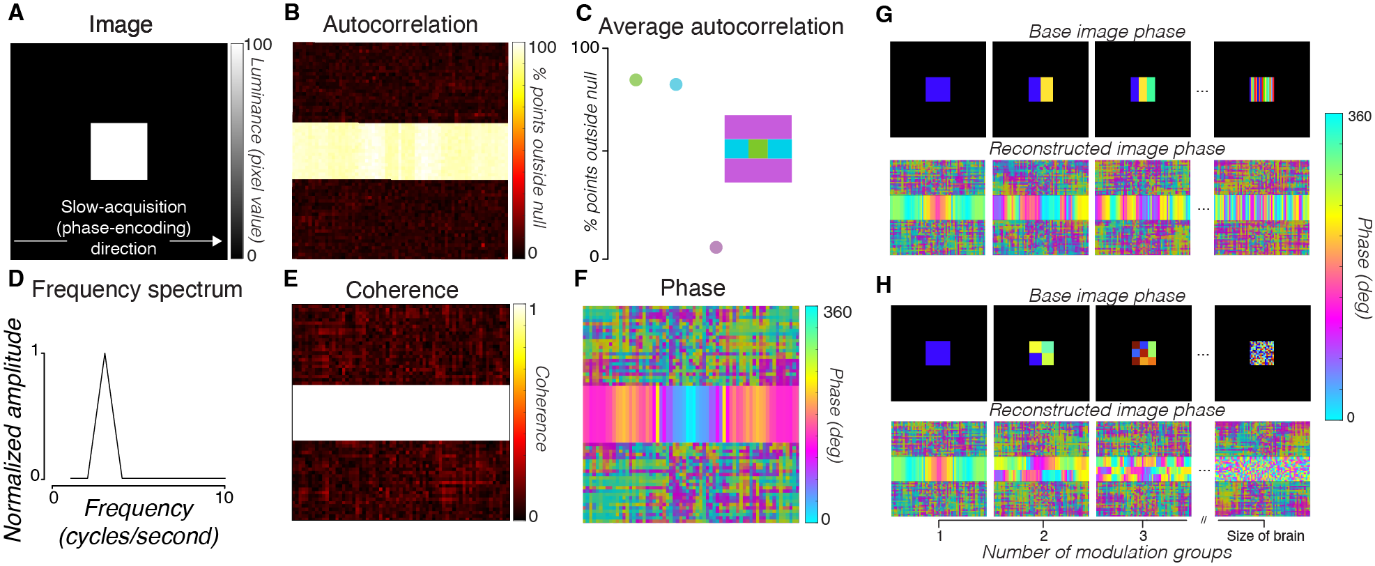
To explain these results, we simulated the line-scan acquisition of a time-varying substrate (Fig 4). The simulated substrate voxels modulated sinusoidally over time (1% amplitude), and the voxels outside the substrate were fixed to zero. We simulated k-space lines acquired at different phases of the modulation. The reconstructed images have the same spatial artifacts as the in vivo measurements (Fig 5). The simulated time series had higher APM levels in voxels along the phase-encoding direction from the brain than not (Fig 5C, voxels in cyan vs. purple areas). The phase of the modulation frequency varies across the phase-encoding direction (Fig 5F), similar to the phase variation in the human data (Fig 3H).
The simulation suggests that the artifacts in the human data arise from slow, widespread physiological processes, such as the cardiac and respiratory cycles. We ran simulations in which we randomized the phase of the modulation between different subregions of the brain. Breaking the assumption of global coherence in the simulation produces a progressively less-ordered phase gradient of the major frequency component along the phase-encoding dimension of the reconstructed image (Fig 5G, H, “reconstructed image phase”). These simulations suggest that a globally coherent modulation is the best match to the in vivo data.
The data and simulations suggest that physiological noise is particularly problematic in line-scan MRI because of the long acquisition time for single images, giving rise to artifacts that spread across the image.

Acknowledgements

No acknowledgement found.