Introduction

For rapid 3D and single-shot Multiband (MB) imaging, the most common method to sample the phase-encoding (PE) plane in k-space is blipped-CAIPIRINHA¹, providing oblique grids with varying SNR efficiency². Sampling on tilted hexagonal (T-Hex) grids³ provides optimal sampling patterns in terms of g-factor noise amplification by maximizing the circle packing density of the lattice⁴, resulting in hexagonal tiling of aliases in the image domain⁵. However, for a given FOV and resolution, T-Hex offers only a discrete set of viable undersampling factors. Yet, when optimising SNR, contrast and effective resolution, it is desirable to choose these parameters flexibly. Here we propose a way of maximizing the packing density, and thus sampling efficiency, for arbitrary undersampling factors - bringing sampling into the Holocene.

Methods

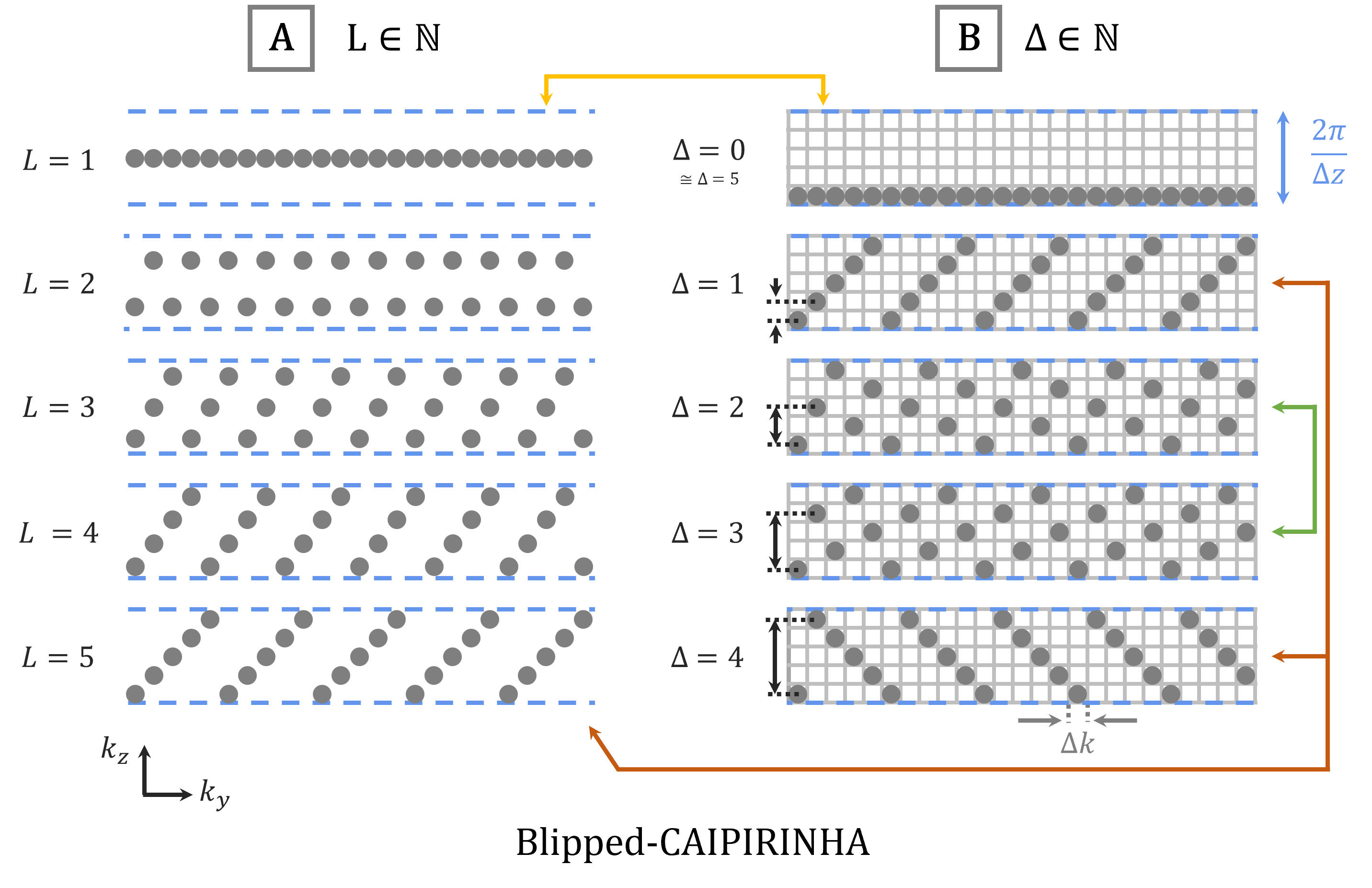
MB encoding requires a lower resolution in z direction than full 3D encoding⁵ (given by the distance $$$Δz$$$ between $$$N$$$ simultaneously excited slices), but the same sampling density. Therefore, this work focuses on MB imaging.

A) Blipped-CAIPIRINHA as introduced initially^1,6, samples k-space on $$$L$$$ distinct planes in through-plane (here z) direction (Figure 1A) with $$$N>L\in\mathbb{N}$$$ and all planes being visited repetitively in monotonically increasing order. This is realized through additional z-gradient-blips after each frequency-encoding (FE) line: $$$L-1$$$ small blips in +z direction and one larger blip -z direction, repeated sequentially.

B) Blipped-CAIPIRINHA’s SNR can be enhanced by shuffling the order of visited k-space planes² (Figure 1B) with $$$Δ\in\mathbb{N}$$$ defining the distance between consecutively visited planes⁷ in multiples of $$$Δk=2π/FOV$$$, i.e., $$$Δ=N/L$$$ where now $$$L\in\mathbb{Q}$$$.

The optimum $$$L$$$ or $$$Δ$$$ for both approaches have so far been determined heuristically. We propose to choose them as real-valued numbers ($$$L, Δ\in\mathbb{R}$$$) and such that the PE grid exhibits maximum circle packing density, $$$D$$$.
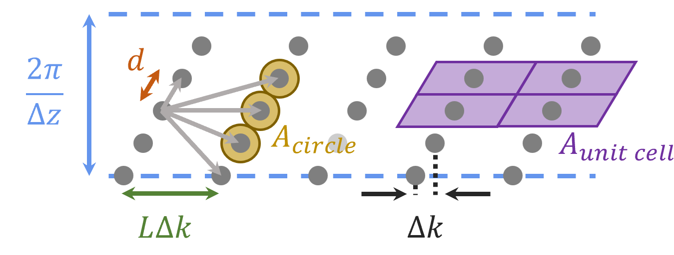
For an oblique lattice (Figure 2), $$$D$$$ is the fraction of the surface covered, if a circle is centred around each lattice point and all circles are of the same dimension and as large as possible without generating overlap. It can be computed as the ratio of the area of one such circle to the area of a primitive unit cell of the lattice:

$$D=\frac{A_{\text{circle}}}{A_{\text{unit cell}}}$$

$$$A_{\text{unit cell}}$$$ is independent of the choice of $$$L$$$ and $$$Δ$$$:

$$A_{\text{unit cell}}=\frac{2\pi\Delta{k}}{\Delta{z}}$$

with the in-plane PE-spacing

$$\Delta k=\frac{2\pi{R_{\text{in-plane}}}}{\text{FOV}_{\text {in-plane}}}$$

and the in-plane undersampling factor $$$R_{\text{in-plane}}$$$.

$$$A_{\text{circle}}$$$ depends on the sampling pattern:

$$A_{\text{circle}}=\frac{\pi}{4}d_{\min}{ }^2$$

where $$$d_{\min}$$$ is the smallest distance between adjacent lattice points and is computed from all possible distances as

$$d_{\min}(L)=\min_{m\in\mathbb{Z}}\left(\sqrt{(m\cdot\Delta{k})^2+\left(\frac{2\pi}{\Delta{z}}\right)^2\left(\frac{m}{L}-\left\lfloor\frac{m}{L}\right\rfloor\right)^2}\right)$$

The optimum sampling pattern (maximum $$$D$$$) maximizes $$$d_{\min}$$$

$$\max_{L\in\mathbb{R}}\left(d_{\min}(L)\right)$$

The total undersampling factor can be chosen freely as $$$R_{\text{total}}=N\cdot{R_{\text {in-plane }}}$$$ where $$$R_{\text{in-plane}}\in\mathbb{R}$$$. In particular, $$$R_{\text{in-plane}}$$$ can take values < 1 if the imaging situation requires/allows for a higher acceleration ($$$N$$$) than total undersampling factor ($$$R_{\text{total}}$$$). The term $$$R_{\text{in-plane}}$$$ is used to conform with previous descriptions of the subject matter, although for $$$L>1$$$ a clear distinction between in-plane and through-plane undersampling is impossible². Matlab code for all computations and creation of figures is available under https://git.cardiff.ac.uk/sapme1/holocenesampling.

Results

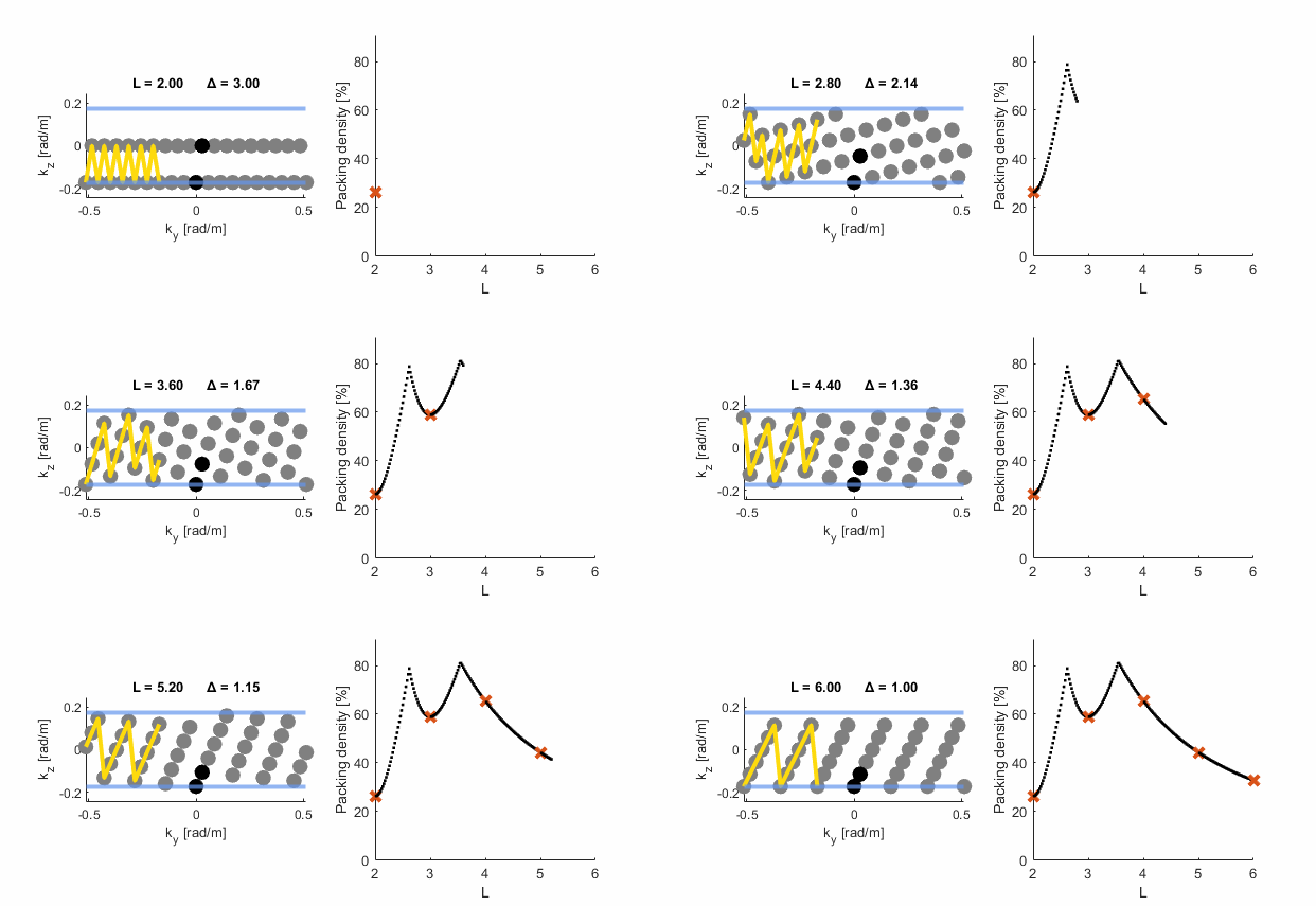
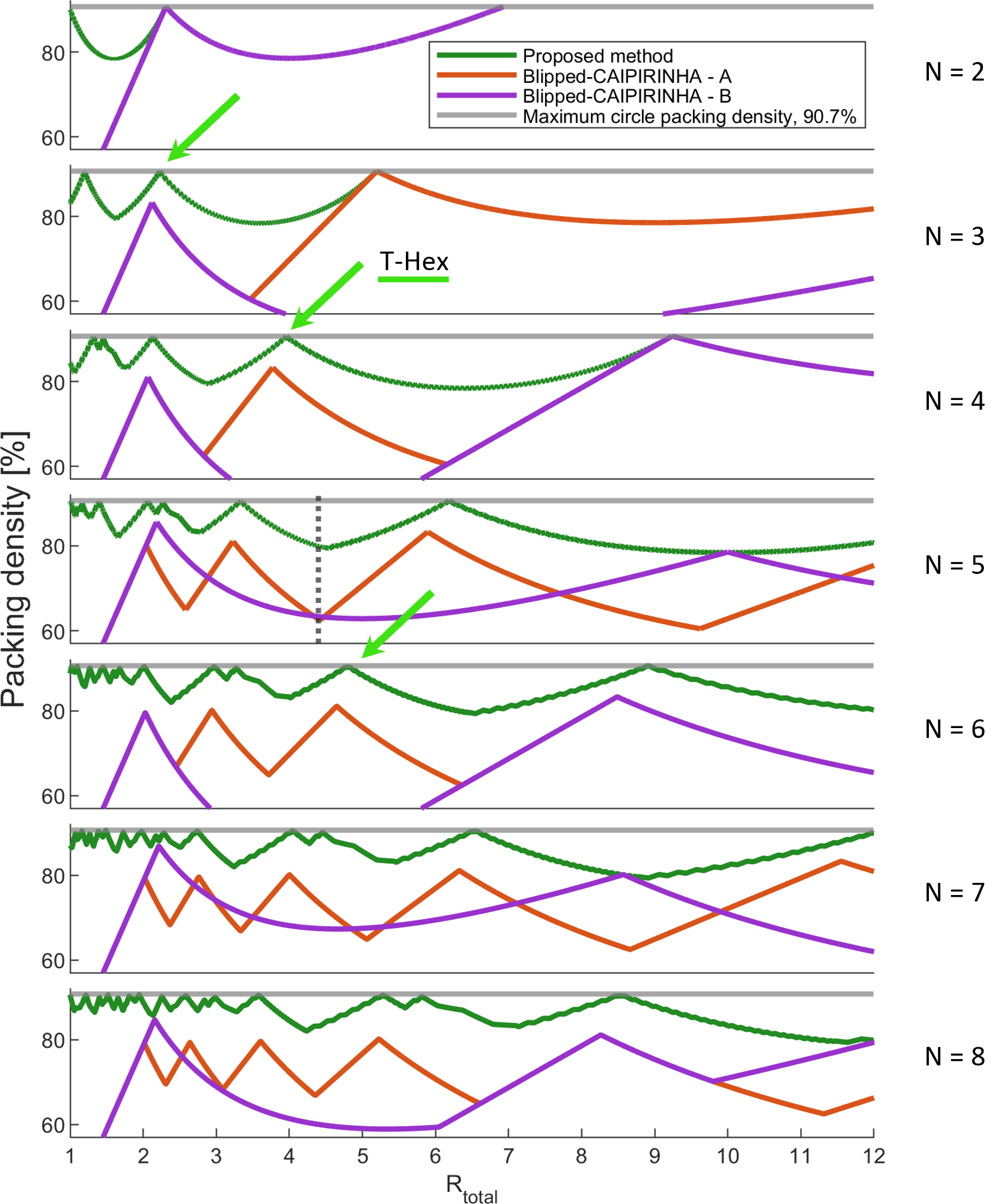
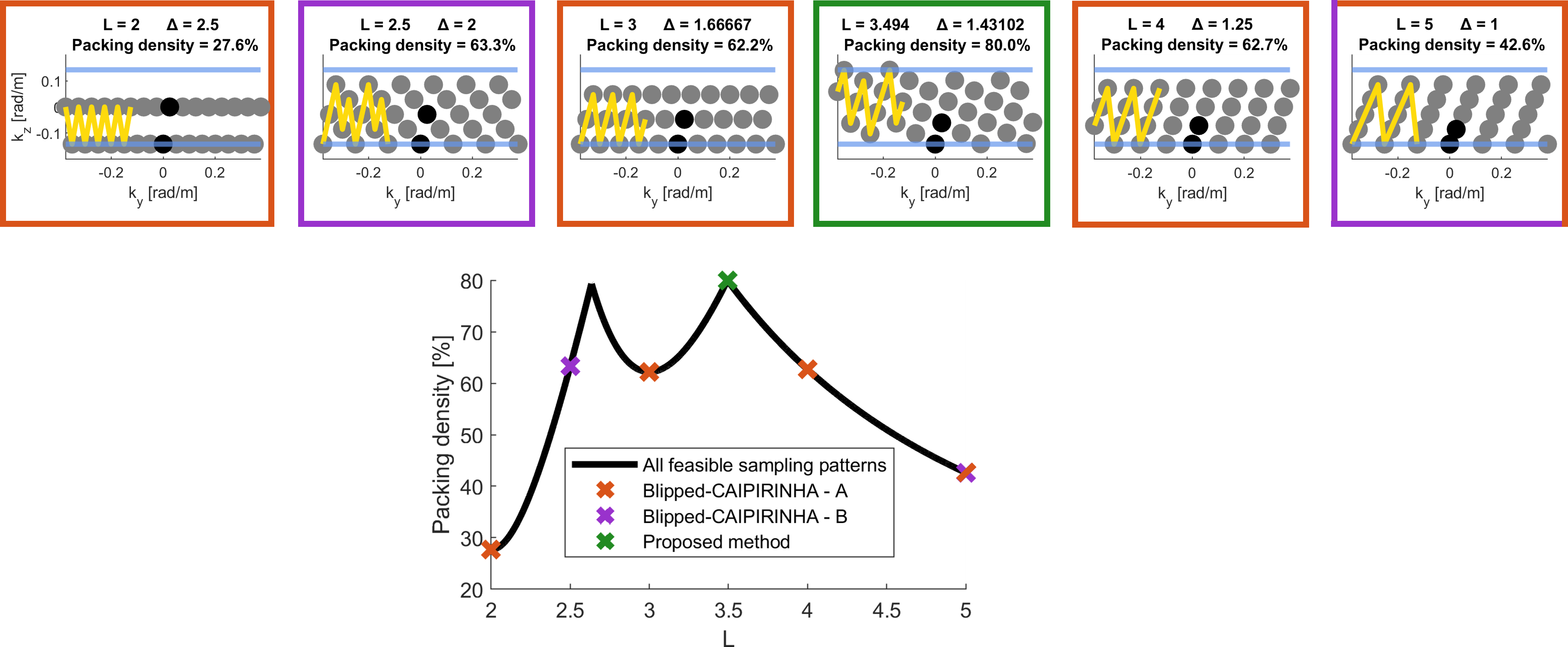
Gif 1 shows feasible grids and resulting $$$D$$$ for fixed imaging parameters ($$$FOV_{\text{in-plane}}=22.0~cm, R_{\text{in-plane}}=1, N=6, \Delta{z}=1.83~cm$$$). Blipped-CAIPIRINHA reaches maximally $$$D=65\%$$$ ($$$L=4$$$), whereas the proposed method reaches $$$D=81\%$$$ ($$$L=3.55$$$).
For a range of scenarios, Figure 3 shows the maximum $$$D$$$ reached with the proposed method and with blipped-CAIPIRINHA, the former outperforming almost always the latter.
For high $$$R_{\text{total}}$$$, both methods yield identical results. The convergence point occurs the earlier, the smaller $$$N$$$ – or in 3D sampling terms, the smaller the k-space volume sampled within one readout. Starting at some (even higher) $$$R_{\text{total}}$$$, the packing density computation as proposed here becomes degenerate as the smallest distance between grid points is larger than the k-space slab that needs to be sampled $$$d_{\min}>2\pi/\Delta z$$$ (here only seen for $$$N=2$$$, where curve stops at $$$R\sim7$$$).
The proposed method coincides with T-Hex whenever optimum hexagonal sampling is feasible, which happens more frequently for lower $$$R_{\text{total}}$$$ and higher $$$N$$$. Figure 4 displays relevant grids for the case marked with a dashed line in Figure 3.

Discussion

The key contribution of our method is that it delivers the maximally feasible packing density of aliases in the image domain regardless of the given imaging parameters. Whereas T-Hex provides the optimum packing density, it is restricted to discrete undersampling factors/readout times. The current work will output T-Hex, wherever possible, and otherwise maximally close patterns. For the $$$N=5$$$ example shown here, T-Hex would provide $$$R_{\text{total}}=6.2,3.3,2.2...$$$ Intermediate undersampling factors might be desirable if $$$R=3.3$$$ requires excessive readout durations (T₂-decay and intra-voxel dephasing) and $$$R=6.2$$$ entails too little SNR, given receive coil geometry, field strength and imaging application.

Acknowledgements

EPSRC (grant EP/M029778/1); The Wolfson Foundation; Wellcome Trust Investigator Award (096646/Z/11/Z); Wellcome Trust Strategic Award (104943/Z/14/Z); Siemens Healthineers;