3279
Automatic Detection of BOLD Activations using a Semi-supervised Bidirectional LSTM Neural Network1Laboratory for Social and Neural Systems Research (SNS Lab), University of Zurich, Zurich, Switzerland, 2Institute for Biomedical Engineering, ETH Zurich and University of Zurich, Zurich, Switzerland
Synopsis
Keywords: fMRI Analysis, Machine Learning/Artificial Intelligence, HiHi fMRI, Data Analysis
Motivation: Because there is significant variability in the hemodynamic response of individuals, fitting a simple function may lead to false negatives (i.e., a bad fit leads to larger residuals than the noise level would dictate).
Goal(s): Develop a robust data-driven based approach for detecting BOLD.
Approach: A semi-supervised automatic detection (SAD) method based on a bidirectional long/short-term memory neural network to find BOLD responses in the entire brain and assess classification performance on simulated fMRI data.
Results: The proposed detection method exhibits robustness across various HRF shapes at realistic contrast-to-noise ratios.
Impact: We proposed a method for detecting BOLD responses in high temporal resolution fMRI data that is based on a Bidirectional long/short-term memory neural network. Classification performance was excellent as tested using simulated data with different HRFs and contrast-to-noise ratios.
Introduction
The most widely used method for detecting BOLD activations in fMRI times-series relies on a general linear model and voxel-wise fits of an assumed haemodynamic response function (HRF) to the data1. Given that the HRF models have few parameters, which may not capture all the details of a BOLD response2 and that there is considerable variability in the BOLD response across sessions, subjects and cortical areas3–5, a model-free signal detection method may be desirable. In the present study, we develop a semi-supervised automatic detection (SAD) method based on a bi-directional long-short term memory (Bi-LSTM) neural network6,7 for detection of BOLD activations, train it on in-vivo data with 75-ms temporal sampling resolution8 and deploy the model on simulated data with different shapes of HRF’s to assess classification performance.Methods
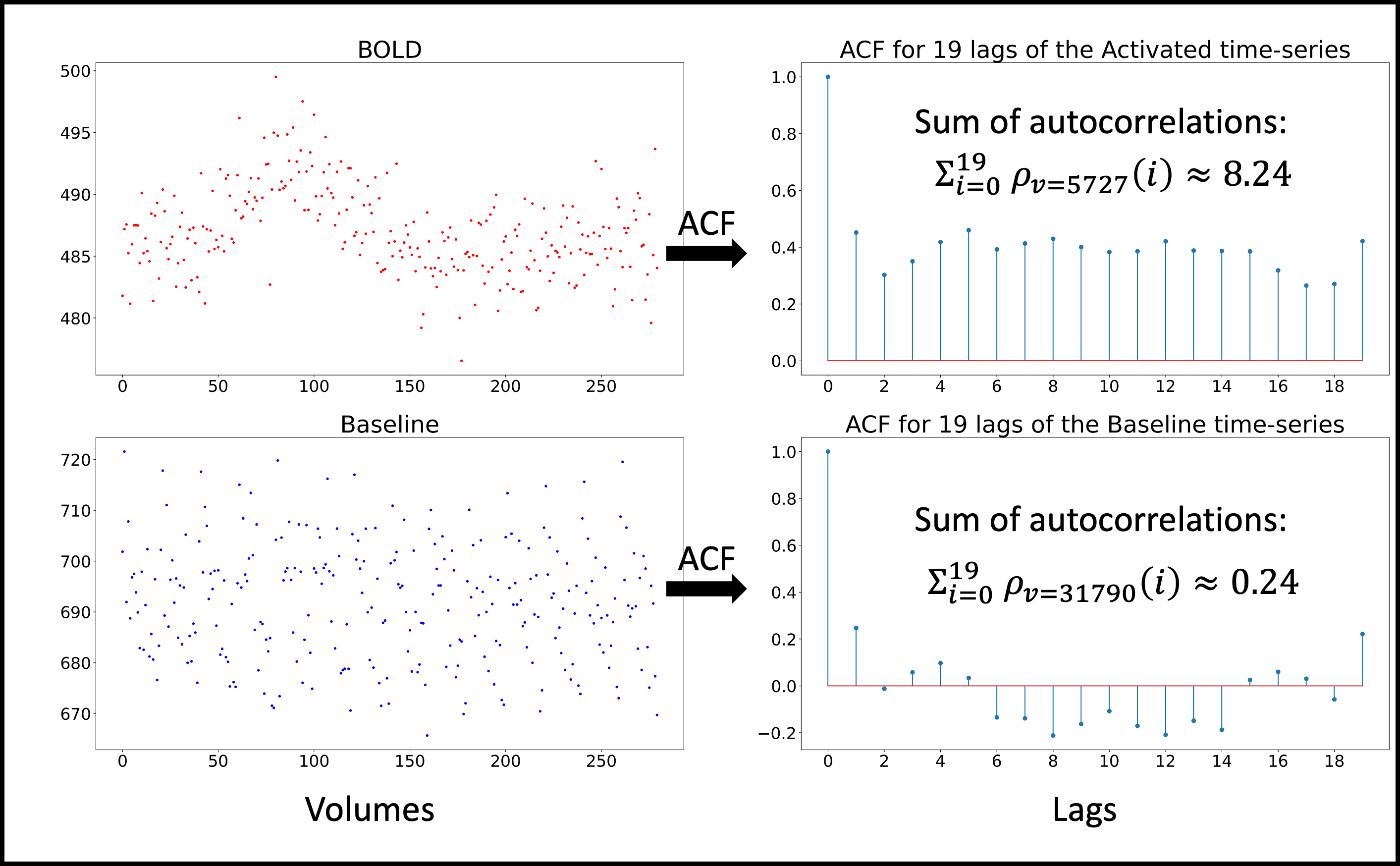
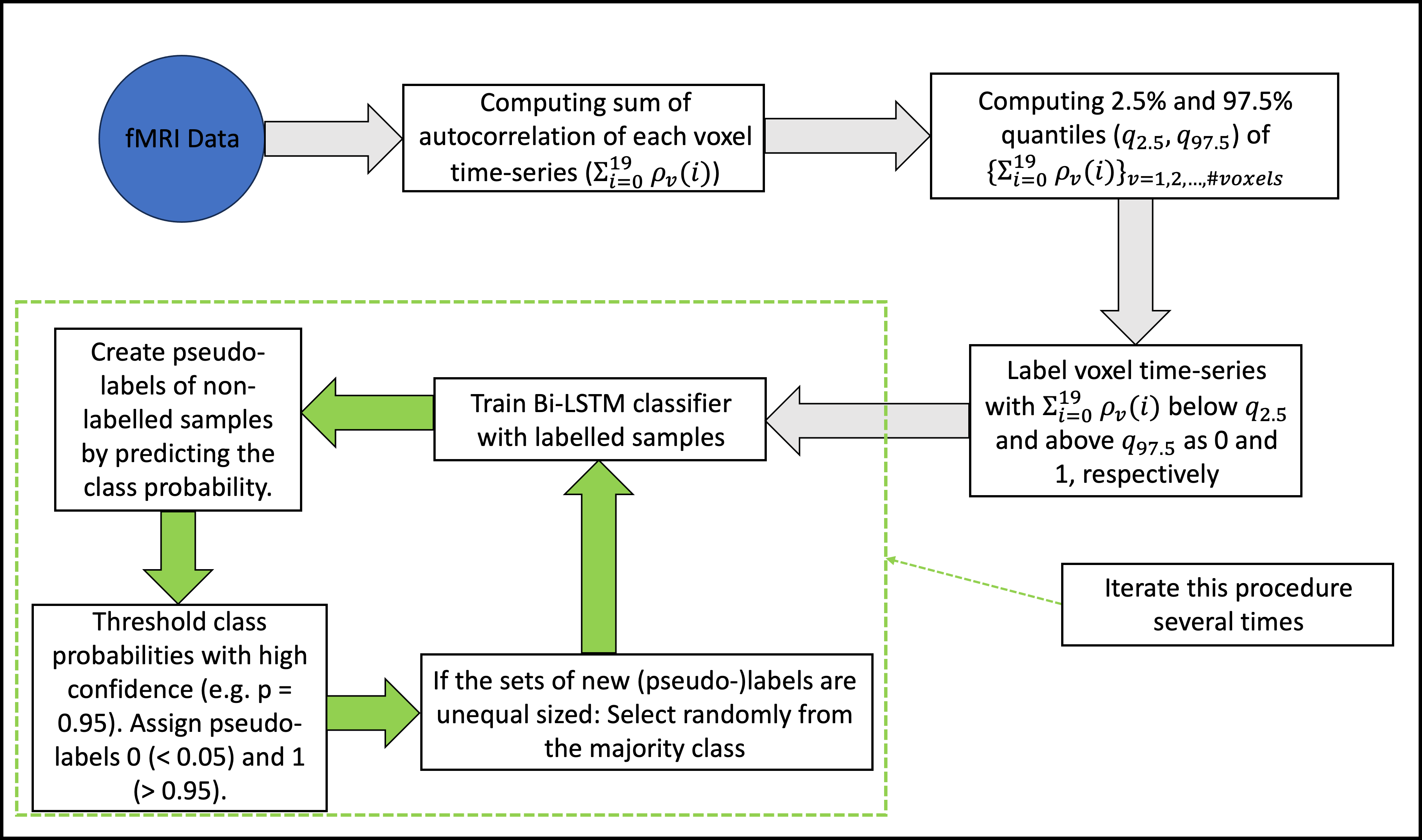
2.1 The proposed semi-supervised automatic detection (SAD) methodThe proposed SAD method consists of three Bi-LSTM blocks with hidden dimensions of 15, 10 and 3, respectively, a batch normalization layer after the first two Bi-LSTM blocks and a fully connected layer with sigmoid activation function to map the output into the scalar interval [0,1]. In total, the network contains 4734 trainable parameters. To avoid manually labelling tens of thousands of voxels, (pseudo-)labels were created in an iterative scheme. First, ‘baseline’ or ‘activation’ labels were assigned voxel-wise based on the 2.5% upper and lower quantiles of the sum of the autocorrelations9 (Fig. 1/2) of the fMRI data, respectively. Subsequently, additional voxels were labelled based on the most confidently predicted label probabilities. At each iteration the neural network was trained using mini-batch (batch size 32) stochastic gradient descent (Adam optimizer10) with a constant learning rate of 0.001 and 50 epochs. To address class imbalance, we introduced a penalization, which emphasizes the difference between activated and non-activated time-series (Eq. 1) and randomly undersample the majority class.
$$ P_{predicted}(v) = \frac{P_{Bi-LSTM NN}(v)}{1+exp(-\Sigma_{i=0}^{19} \rho_v(i))} \quad (1) $$
2.2 Data acquisition
We used the HiHi fMRI data11 which had 75-ms temporal resolution and were acquired on a 7T MAGNETOM Terra scanner (Siemens Healthcare, Erlangen, Germany) with a single channel transmit and 32ch receive head coil (Nova Medical Inc., MA, United States) using a 2D EPI12 sequence combined with multiband acceleration factor of 313,14 that had a TR of 1.5 s. The task involved fixating on a small white cross in the centre of a gray background, which turned into a checkerboard flickering at 8 Hz for 375 ms approximately every 21 seconds8.
2.3 Data analysis
The data were analysed with custom-made Matlab (version 2021a) and Python (version 3.9.12) scripts, SPM121 and PyTorch (version 2.0.1). The in-vivo fMRI data were 3D rigid-body aligned to the first EPI volume, followed by voxel-wise signal detrending using a second-degree polynomial regression. Afterwards, the data were reshuffled according to the HiHi reordering algorithm8,11. We assessed classification performance using simulated data with different shapes of HRFs and different contrast-to-noise ratios (CNR) using SPM's two Gamma function model1,15 (Eq. 2) and Gaussian signal-independent noise.
$$ h(t) = A [t^{\alpha_1 -1}exp(-\beta_1 t)\beta_1^{\alpha_1}/\Gamma(\alpha_1)- c t^{\alpha_2 -1}exp(-\beta_2 t)\beta_2^{\alpha_2}/\Gamma(\alpha_2)] \quad (2) $$
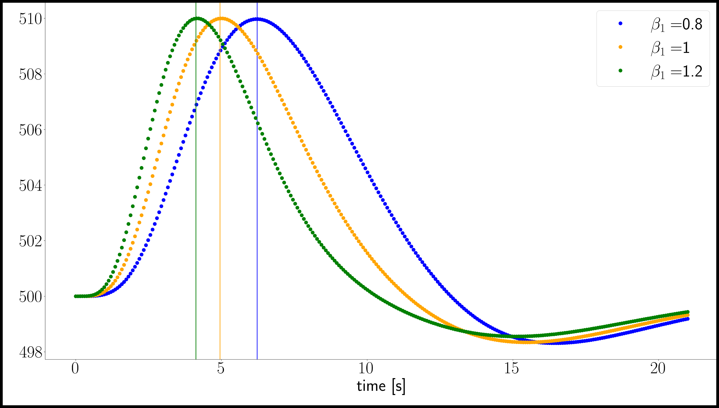
Figure 3 shows some examples of simulated hemodynamic response functions for varying $$$\beta_1$$$ (Eq. 2) with base signal intensity of 500.
Results
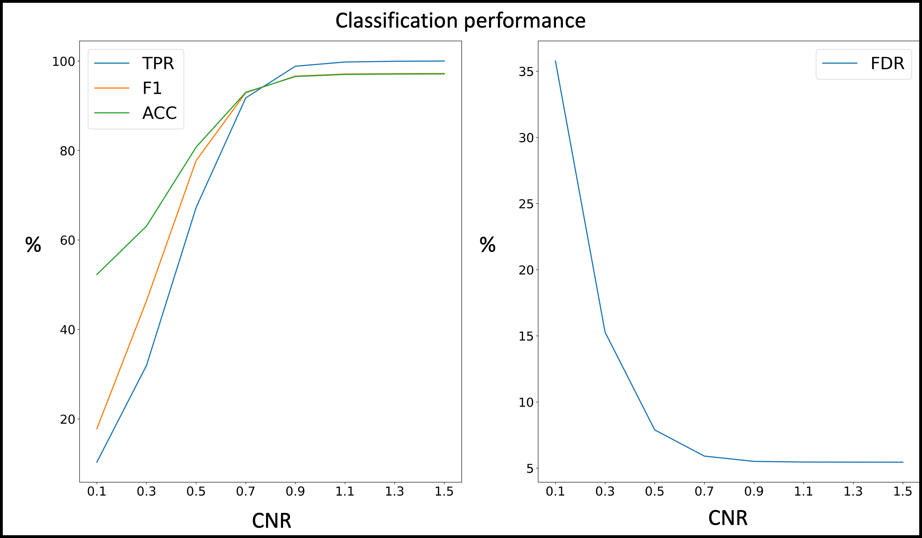
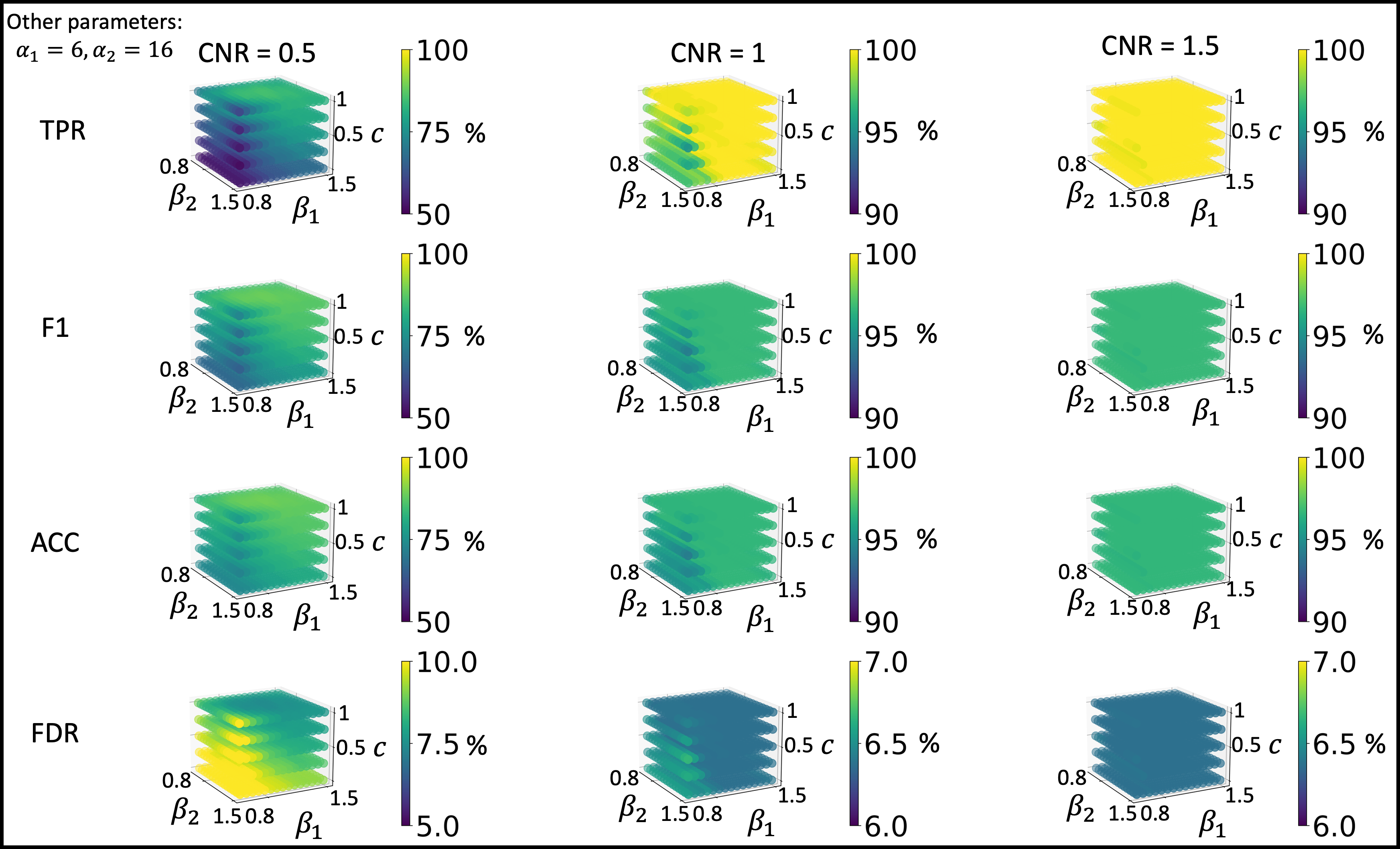
In Figure 4, four classification performance scores are depicted as percentages across varying CNRs, while the temporal signal-to-noise ratio (tSNR) is kept at 100. All scores plateau around a CNR of 1.1.Figure 5 provides the (color-coded) true positive rate (TPR) for different shapes of the HRF as a function of the parameters $$$\beta_1, \beta_2$$$ and $$$c$$$, where the latter two control the undershoot and the former the peak and $$$\alpha_1,\alpha_2$$$ kept constant at their default values. Unsurprisingly, the worst performance occurs at the lowest CNR. As in Figure 4, classification scores level off around a CNR of 1.
Discussion and Conclusion
We have proposed a semi-supervised automatic detection (SAD) method to identify BOLD responses. The method is based on a bidirectional LSTM neural network, which was trained and fine-tuned iteratively. For realistic CNR levels of in-vivo data the method demonstrated excellent classification performance on simulated data. Future work will deploy the model on additional in-vivo data, investigate whether the model can be generalized across different individuals or repeated scans or needs re-training. Because the method relies on fMRI data with high temporal sampling resolution (here 75 ms), further work will also assess how sampling rate impacts performance.Acknowledgements
No acknowledgement found.References
1. Friston Karl J., Ashburner John T., Kiebel Stefan J., Nichols Thomas E., Penny William D. Statistical Parametric Mapping: The Analysis of Functional Brain Images. 1st ed. Academic Press; 2007.
2. Polimeni JR, Lewis LD. Imaging faster neural dynamics with fast fMRI: A need for updated models of the hemodynamic response. Prog Neurobiol. 2021;207. doi:10.1016/j.pneurobio.2021.102174
3. McGonigle DJ, Howseman AM, Athwal BS, Friston KJ, Frackowiak RSJ, Holmes AP. Variability in fMRI: An examination of intersession differences. Neuroimage. 2000;11(6 I):708-734. doi:10.1006/nimg.2000.0562
4. Aguirre GK, Zarahn E, D’esposito M. The Variability of Human, BOLD Hemodynamic Responses. Neuroimage. 1998;8(4):360-369. doi:10.1006/nimg.1998.0369
5. Handwerker DA, Ollinger JM, D’Esposito M. Variation of BOLD hemodynamic responses across subjects and brain regions and their effects on statistical analyses. Neuroimage. 2004;21(4):1639-1651. doi:10.1016/j.neuroimage.2003.11.029
6. Hochreiter S, Schmidhuber J. Long short-term memory. Neural Comput. 1997;9(8):1735-1780.
7. Goos G, Hartmanis J, Van J, et al. LNCS 3697 - Artificial Neural Networks: Formal Models and Their Applications … ICANN 2005.; 2005.
8. Schmidt T, Vannesjo SJ, Sommer S, Nagy Z. fMRI with whole-brain coverage, 75-ms temporal resolution and high SNR by combining HiHi reshuffling and multiband imaging. Magn Reson Imaging. Published online November 2023. doi:10.1016/j.mri.2023.06.015
9. Brockwell PJ, Davis RA. Springer Texts in Statistics Introduction to Time Series and Forecasting. http://www.springer.com/series/417
10. Kingma DP, Ba J. Adam: A Method for Stochastic Optimization. Published online December 22, 2014. http://arxiv.org/abs/1412.6980
11. Nagy Z, Hutton C, David G, et al. HiHi fMRI: a data-reordering method for measuring the hemodynamic response of the brain with high temporal resolution and high SNR. Cerebral Cortex. Published online September 28, 2022. doi:10.1093/cercor/bhac364
12. Schmitt F, Stehling MK, Turner R. Echo-Planar Imaging. 1st ed. Springer Berlin Heidelberg; 1998.
13. Larkman DJ, Hajnal J V, Herlihy AH, Coutts GA, Young IR, Sta Ehnholm G. Use of Multicoil Arrays for Separation of Signal from Multiple Slices Simultaneously Excited. Magn Reson Imaging. 2001;13(2):313-317. doi:10.1002/1522-2586(200102)13:2<313::aid-jmri1045>3.0.co;2-w
14. Moeller S, Yacoub E, Olman CA, et al. Multiband multislice GE-EPI at 7 tesla, with 16-fold acceleration using partial parallel imaging with application to high spatial and temporal whole-brain FMRI. Magn Reson Med. 2010;63(5):1144-1153. doi:10.1002/mrm.22361
15. Martin A. Lindquist, Ji Meng Loh, Lauren Y. Atlas, Tor D. Wager. Modeling the Hemodynamic Response Function in fMRI: Efficiency, Bias and Mis-modeling. Neuroimage. 2012;45:187-198.
Figures