3203
Testing the utility of Dynamic Susceptibility Contrast (DSC)-Perfusion toolbox for mapping the characteristics of mouse brain perfusion1Centre for Advanced Imaging, The University of Queensland, Brisbane, Australia
Synopsis
Keywords: Contrast Agents, DSC & DCE Perfusion
Motivation: Perfusion studies using DSC-MRI offer insights into vascular aspects of cerebral pathophysiology by allowing us to estimate viable perfusion characteristics.
Goal(s): Previous studies have shown successful implementation of DSC MRI toolbox to characterise human brain perfusion, but its application to animal data remains unexplored. Our goal is to characterize perfusion parameters in mouse model using DSC-MRI-toolbox.
Approach: We slightly modified and implemented DSC-MRI-toolbox to meaure CBV, CBF and MTT in different regions of mouse brain such as cortex, hippocampus and thalumus.
Results: Initial data analysis shows a successful implementation of the DSC-MRI-toolbox and allowing us to estimate perfusion parameters in preclinical data.
Impact: A successful implementation of DSC-MRI toolbox in mouse models will allow us to estimate perfusion parameters such as CBV, CBF, MTT and CBV with leakage correction, which will be important for characterising tissue viability in stroke and brain injury models.
Introduction
DSC-weighted MRI is a widely used method for the quantification of cerebral perfusion and accurate quantification of these parameters has multiple clinical applications1, including identification and evaluation of ischemic stroke prior to treatment, the diagnosis of tumours or as biomarkers for the progression of Alzheimer’s disease2-3. It is possible to extract perfusion-related parameters such as Cerebral Blood Flow (CBF), Cerebral Blood Volume (CBV) and Mean Transit Time (MTT) which can be estimated relatively4 Based on tracer kinetic modelling, these hemodynamic parameters can be extracted using DSC-MRI, which can be solved using deconvolution-based methods2,5. To accurately estimate perfusion parameters, we need to have an understanding of reliable arterial input function (AIF)2,4,6. This tool has been successfully implemented in clinical imaging, but their use in preclinical imaging is yet to be explored. In this study, we aim to implement DSC MRI Toolbox to characterise mouse brain perfusion, with a view to use it in the future to better understand pathological mechanisms of various diseases using transgenic mouse models7.Methods
Experimental Setup:Perfusion MRI data was obtained from a method development scanning session, with approval from the Institutional Animal Ethics Committee. Perfusion data from a single mouse was obtained using Biospec 9.4T preclinical MRI (Bruker Inc, Ettlingen, Germany) using a cryogenically cooled coil for transmission and signal reception and BGA-12S HP gradient. The mouse was scanned under 0.5% isoflurane in combination of 2:1 Air:O2 with a constant infusion of 0.1 mg/Kg/hr medetomidine, with the body temperature maintained at 36°-37° using warm water circulation8. DSC perfusion used 0.5 mmol/kg Gd-based contrast agent delivered through the tail vein as a bolus 50 sec after the baseline scan started.
Data Acquisition and Processing:
DSC data was acquired using a 2D EPI gradient echo sequence in Paravision 6.0.1. The imaging parameters were TR=400ms, TE=14ms9 with image resolution of 0.25x0.25x0.7 mm3, 11 slices with a total of 1350 time volumes. MR images were exported to DICOM and converted into NIFTI using AFNI toolbox. The first 600 volumes were analyzed using the DSC-MRI toolbox. Modifications were made in toolbox to extract the DSC-Perfusion parameter maps into NIFTI to enable analysis using FSL and ITK-SNAP. Perfusion leakage was not expected in this healthy control mouse, but fitting leakage correction for CBV10 was retained to establish the baseline for future studies using animal models.
Results
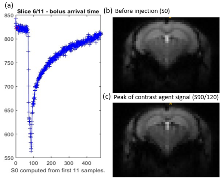
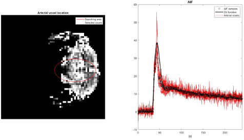
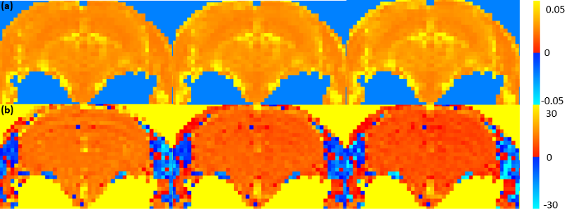
Figure 1 shows the signal intensity in the selected slice along the duration of data acquisition. The bolus of the contrast agent was injected 50 sec after the scan initiation. Out of the 11 slices acquired, being the middle slice, we chose slice 6 to create a mask as our Region of Interest for the AIF Selection. A time-series data of image intensity showed a decrease in signal following the arrival of bolus11 in the brain (Figure 1a). Figure 1b shows the signal intensity before contrast injection, whereas Figure 1c shows the signal intensity in the same slice after contrast injection.Figure 2a shows the region that has been selected for the AIF. Figure 2b shows time series of the AIF from this region for calculating the perfusion parameters The perfusion maps CBF and MTT are shown in Figure 3a and 3b, respectively. Three columns exhibit the different convolution methods namely singular value decomposition (SVD), constrained-SVD (cSVD) and optimized-SVD (oSVD)11. Consistent CBF and MTT are observed with the different convolution methods, but oSVD shows a slight decrease in MTT compared to its counterparts.
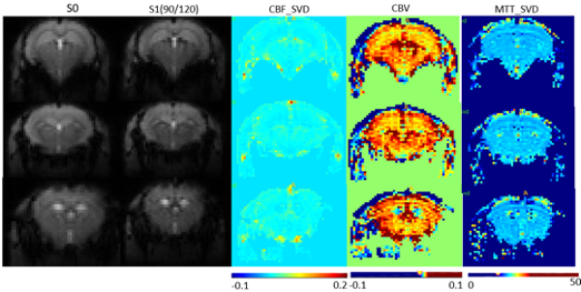
Figure 4 shows the DSC MRI data and calculated perfusion parameters for three slices in the middle of the brain, represented by three rows. The first column represents baseline images prior to contrast agent injection; the second column shows signal drop post-bolus arrival. Columns 3 and 5 respectively show CBF and MTT estimation using the SVD method. Column 4 shows the CBV maps following bolus arrival and changes to the Blood Volume can be observed in hippocampal region.
Discussion
DSC-toolbox generates plots for CBV, CBF, MTT and with correction for any potential contrast agent leakage12. In our study, we implement this toolbox in mouse models to estimate hemodynamic characteristics such as CBV, CBF and MTT. Our preliminary results demonstrate the robustness of this method in accurately quantifying essential hemodynamic parameters, specifically CBV, CBF, and MTT. Successful implementation in a single test subject shows the possibility of reproducing these results in multiple datasets. Few other studies demonstrate the possibility of estimating DSC-perfusion parameters using Python-based-toolbox in mouse models which can be explored and implemented in mouse models5.Acknowledgements
We thank Dr G Leinenga for providing the mouse test data. We acknowledge the support from the Australian National Imaging Facility for the operation of 9.4T MRI at The University of Queensland. DSC MRI toolbox was sourced from https://github.com/marcocastellaro/dsc-mri-toolbox.References
- Cohen-Adad, J. et al. Open-access quantitative MRI data of the spinal cord and reproducibility across participants, sites and manufacturers. Sci Data 8, 219 (2021).
- Peruzzo, D., Bertoldo, A., Zanderigo, F. & Cobelli, C. Automatic selection of arterial input function on dynamic contrast-enhanced MR images. Computer Methods and Programs in Biomedicine 104, e148–e157 (2011).
- Lee, D., Le, T. T., Im, G. H. & Kim, S.-G. Whole-brain perfusion mapping in mice by dynamic BOLD MRI with transient hypoxia. J Cereb Blood Flow Metab 42, 2270–2286 (2022).
- Fernández-Rodicio, S. et al. Perfusion-weighted software written in Python for DSC-MRI analysis. Front. Neuroinform. 17, 1202156 (2023).
- Buxton, R. B. et al. A general kinetic model for quantitative perfusion imaging with arterial spin labeling. Magnetic Resonance in Med 40, 383–396 (1998).
- Mouridsen, K., Christensen, S., Gyldensted, L. & Østergaard, L. Automatic selection of arterial input function using cluster analysis. Magnetic Resonance in Med 55, 524–531 (2006).
- Jonckers, E. et al. Different anesthesia regimes modulate the functional connectivity outcome in mice: Anesthesia and Functional Connectivity Outcome in Mice. Magn. Reson. Med. 72, 1103–1112 (2014).
- To, X. V., Vegh, V. & Nasrallah, F. A. Towards data-driven group inferences of resting-state fMRI data in rodents: Comparison of group ICA, GIG-ICA, and IVA-GL. Journal of Neuroscience Methods 366, 109411 (2022).
- Jin, S., Han, S., Stoyanova, R., Ackerstaff, E. & Cho, H. Pattern recognition analysis of dynamic susceptibility contrast (DSC)‐MRI curves automatically segments tissue areas with intact blood–brain barrier in a rat stroke model: A feasibility and comparison study. Magnetic Resonance Imaging 51, 1369–1381 (2020).
- Østergaard, L. et al. High resolution measurement of cerebral blood flow using intravascular tracer bolus passages. Part II: Experimental comparison and preliminary results. Magnetic Resonance in Med 36, 726–736 (1996).
- Østergaard, L., Weisskoff, R. M., Chesler, D. A., Gyldensted, C. & Rosen, B. R. High resolution measurement of cerebral blood flow using intravascular tracer bolus passages. Part I: Mathematical approach and statistical analysis. Magnetic Resonance in Med 36, 715–725 (1996).
- Zanderigo, F., Bertoldo, A., Pillonetto, G. & Cobelli, C. Nonlinear Stochastic Regularization to Characterize Tissue Residue Function in Bolus-Tracking MRI: Assessment and Comparison With SVD, Block-Circulant SVD, and Tikhonov. IEEE Trans. Biomed. Eng. 56, 1287–1297 (2009).
Figures