3123

Applications of the likelihood function for dynamic contrast enhanced MRI

Karl Landheer¹, Marilena Preda¹, Thomas Cook², Johnathon R Walls¹, Mary Germino¹, and Leigh Spencer Noakes¹
¹Regeneron Pharmaceuticals, Inc, Tarrytown, NY, United States, ²University of Massachusetts, Amherst, MA, United States

Synopsis

Keywords: Data Processing, Perfusion

Motivation: Least squares can provide biased and inefficient estimations of pharmokinetic parameters in certain circumstances.

Goal(s): To develop a more efficient method to extract pharmokinetic parameters as well as the limit on the precision of those parameters.

Approach: The likelihood function for multi-channel receive dynamic contrast enhanced MRI was used to develop a method to extract pharmokinetic parameters.

Results: The proposed maximum likelihood estimator method has substantially less bias than the typical least squares method. For the input parameters investigated the maximum likelihood estimated pharmacokinetic parameters had standard deviations within 10% or less of their fundamental lower bound.

Impact: The developed tool provides nearly efficient pharmokinetic estimations, thereby providing an improved method over the standard least squares approach, as well as demonstrating the limited utlility of future machine learning and other methods attempting to solve this problem.

Introduction

The typical method of estimating pharmacokinetic parameters from dynamic contrast enhanced- (DCE-) MRI involves fitting a model to the tissue-concentration curves via non-linear least squares¹ (NLLS). Alternative methods based on machine learning^2,3 Bayesian statistics⁴, and maximum likelihood estimation (MLE), which relied on the assumption of tracer concentrations being sampled from a normal distribution⁶ have been used. We develop a MLE method without this assumption and compare its performance to NLLS with synthetic and in vivo data. Additionally, we use the likelihood function to derive a form for the Cramér-Rao lower bounds (CRLBs), to test how close the standard deviations come to their fundamental limit (i.e., efficiency^5,7).

Methods

The signal for a typical DCE-MRI gradient echo sequence reconstructed with sum-of-squares is

$$A(t)=A_0\sqrt{2m}\left[ \dfrac {1-cos\theta \space exp(-TR\cdot R_1^0)} {1-exp(-TR\cdot R_1^0)} \right] \left[ \dfrac {1-\space exp\left(-TR\cdot \left[rC_t(t)+ R_1^0\right]\right) } {1-cos\theta \space exp\left(-TR\cdot \left[rC_t(t)+ R_1^0\right]\right) } \right], \label{myequation} \tag{1}$$

where A₀ is the baseline signal amplitude, $$$\theta$$$ is the flip angle (30°), m is the number of quadrature receiver coils, TR is the repetition time (6.5 ms), t is time (0.533 s per time point), r is the relaxivity of the contrast agent (2.28 1/(s⋅mM)⁸), $$$R_1^0$$$ is the baseline tissue relaxation rate (1/T1, 0.42 ± 0.02 1/s, measured in 12 mice kidneys), and $$$C_t(t)$$$ is the contrast agent concentration in the tissue. We use the extended Toft’s model⁹ to parameterize $$$C_t(t)$$$, although other models^10–13 can be used:

$$C_t(t)=v_pC_p(t)+\int_{0}^{t}C_p(t)\space exp\left( \frac {K_t} {v_e}[t-\tau]\right)d\tau, \label{myequation2} \tag{2}$$

where $$$K_t$$$, $$$v_e$$$, and $$$v_p$$$, are the pharmacokinetic parameters¹⁴.
Monte Carlo simulations were performed with A₀ = 1, $$$K_t$$$ = 0.4 1/s, $$$v_e$$$ = 0.6, $$$v_p$$$ = 0.1 (representative of a mouse kidney cortex) for $$$SNR \equiv \frac {A(t=0)} {\sigma} \in \{4,8,16\}$$$ and $$$ m \in \{1,8,32,64\}$$$, with noise being sampled 2000 times from a non-central χ distribution, and $$$ \sigma $$$ being the standard deviation of the noise. A simulation was performed for each set of parameters, as well as increasing each of the four estimated parameters by 0.05 to estimate the Jacobian of the expectation values of the estimator.
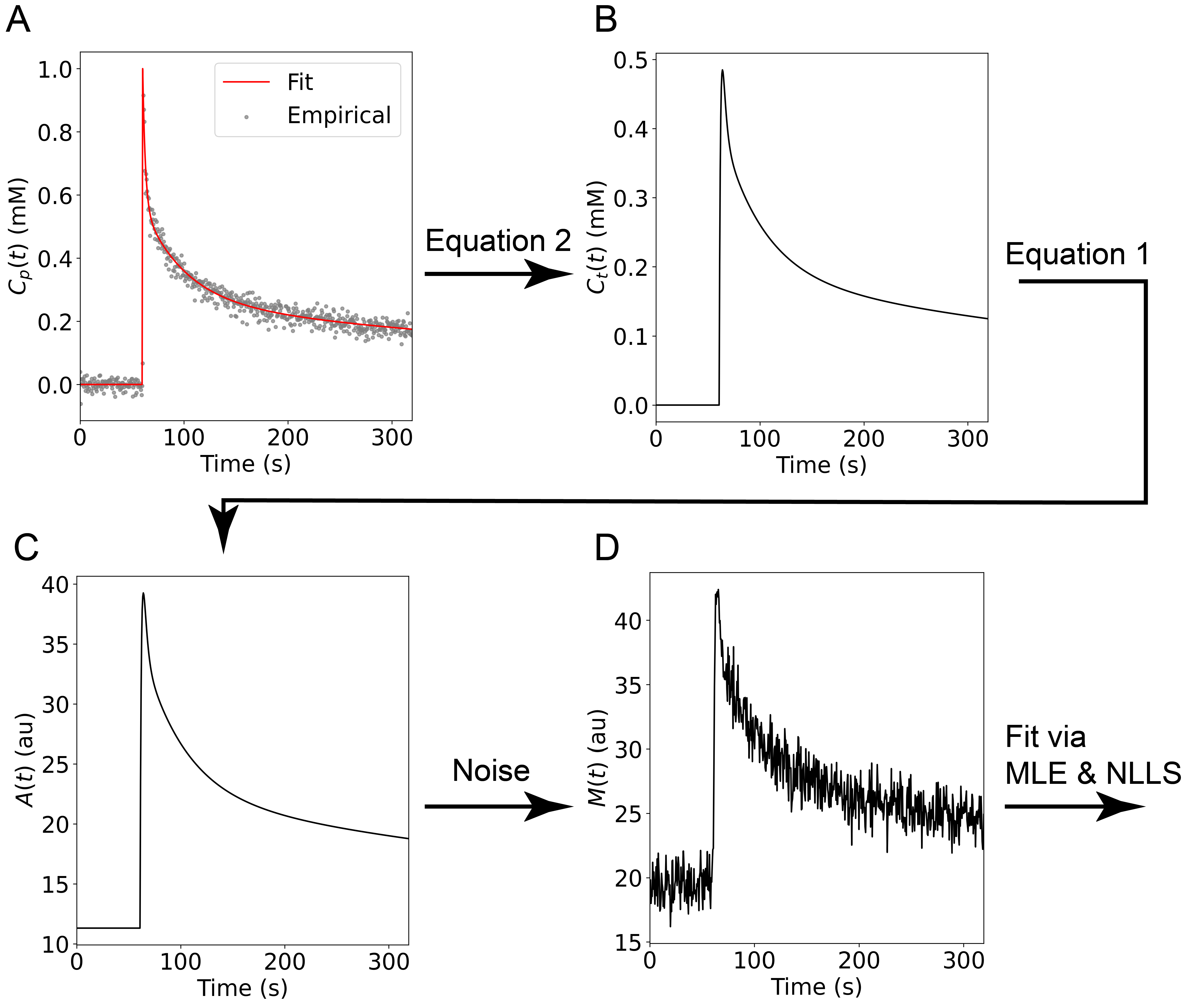
The feeding contrast plasma concentration curve, $$$C_p(t)$$$, was obtained by fitting a measured concentration curve in one animal to a tri-exponential function (similar to the typical bi-exponential^12,15,16):

$$ C_p(t)=\left[ P_1exp\left(\frac {-t} {P_2}\right)+P_3exp\left(\frac {-t} {P_4}\right)+P_5exp\left(\frac {-t} {P_6}\right)\right]H(t-P_7), \label{myequation3} \tag{3}$$

where H is the Heaviside function and $$$P_{1-7}$$$ were fitted parameters found to be 0.43 mM, 2.63 s, 0.30 mM, 40.38 s, 0.27 mM, 626.57 s and 61.30 s, respectively. $$$ C_p(t)$$$ was then used to generate the synthetic data as outlined in Figure 1.

For each of the 2000 Monte Carlo iterations $$$\beta$$$ was estimated by: 1) NLLS¹, and 2) MLE by numerically maximizing the log-likelihood function for phased-array sum-of-squares reconstructed MRI¹⁷

$$ log\left( \mathscr{L}_x\left[ M(t),A(t),\sigma,m\right]\right)=\sum_{n=1}^N log\left(\frac{A^{1-m}_n} {\sigma^2}\right)+log(M_n^m)-\left( \frac{M_n^2+A_n^2} {2\sigma^2}\right)+\left| \frac{M_nA_n} {\sigma^2}\right|+log\left( ^eI_{m-1}\left( \frac {M_nA_n} {\sigma^2}\right) \right), \label{myequation4} \tag{4} $$
where N is the number of data points (600), M(t) is the synthetic noisy signal and $$$ ^eI_{m-1}$$$ is the exponentially scaled modified (m-1)^th order Bessel function of the first kind, used over the modified Bessel function for numerical stability purposes. All numerical optimizations were performed using the Nelder-Mead method (SciPy version 1.4.1) with 10 iterations of the basin hopping algorithm¹⁸. Simulated signals were fit in the signal domain¹¹, as opposed to the concentration domain, since it greatly simplifies the calculation of the likelihood function by avoiding the need to a priori estimate the baseline signal. The CRLB for a biased estimator is^19,20

$$ SD(\beta_i)\geq CRLB(\beta_i)\equiv\sqrt{\left[ \phi(\beta)F^{-1}\phi(\beta)^T \right]_{i,i}}, \label{myequation5} \tag{5}$$
where $$$\phi(\beta)=\frac{\partial\left( \beta+b(\beta)\right)} {\partial\beta }$$$, and $$$ b(\beta)$$$ is the bias, $$$ b(\beta)=E\left[\widehat{\beta}\right] - \beta$$$. For a non-central χ distribution the Fisher information matrix is¹⁷

$$ F_{i,j}=\frac{1} {\sigma^2}\sum_{n=1}^N\frac{\partial A_n} {\partial \beta _j}\frac{\partial A_n} {\partial \beta _i}\left[-\frac{A_n^2}{\sigma^2}+\frac{A^{1-m}_n}{\sigma^4}\int_{0}^{\infty}M_n^{m+2}\frac{^eI_m^2\left( \frac{M_nA_n}{\sigma^2}\right)}{^eI_{m-1}\left( \frac{M_nA_n}{\sigma^2}\right)}exp\left(-\frac{M_n^2+A_n^2} {2\sigma^2}+\left| \frac{M_nA_n}{\sigma^2}\right| \right)dM \right]. \label{myequation6} \tag{6}$$

The standard deviations were calculated via the Monte Carlo simulations with outliers excluded via Tukey’s method^17,21 and compared to the CRLBs.
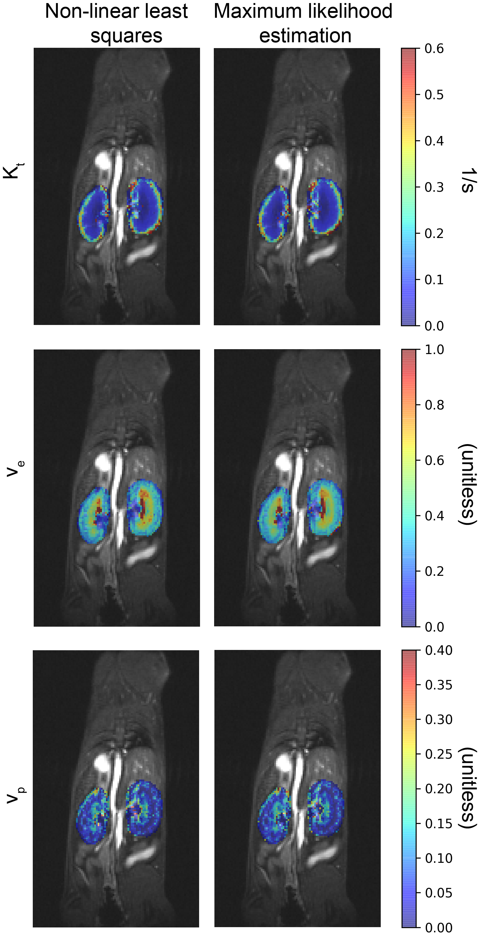
One mouse with m = 1 receive coils was scanned with identical acquisition parameters to the simulations with a Bruker 7T Avance Neo, single transmit/receive coil, and pixel-wise pharmacokinetic maps of the kidneys were created with both MLE and NLLS.

Results and Conclusions

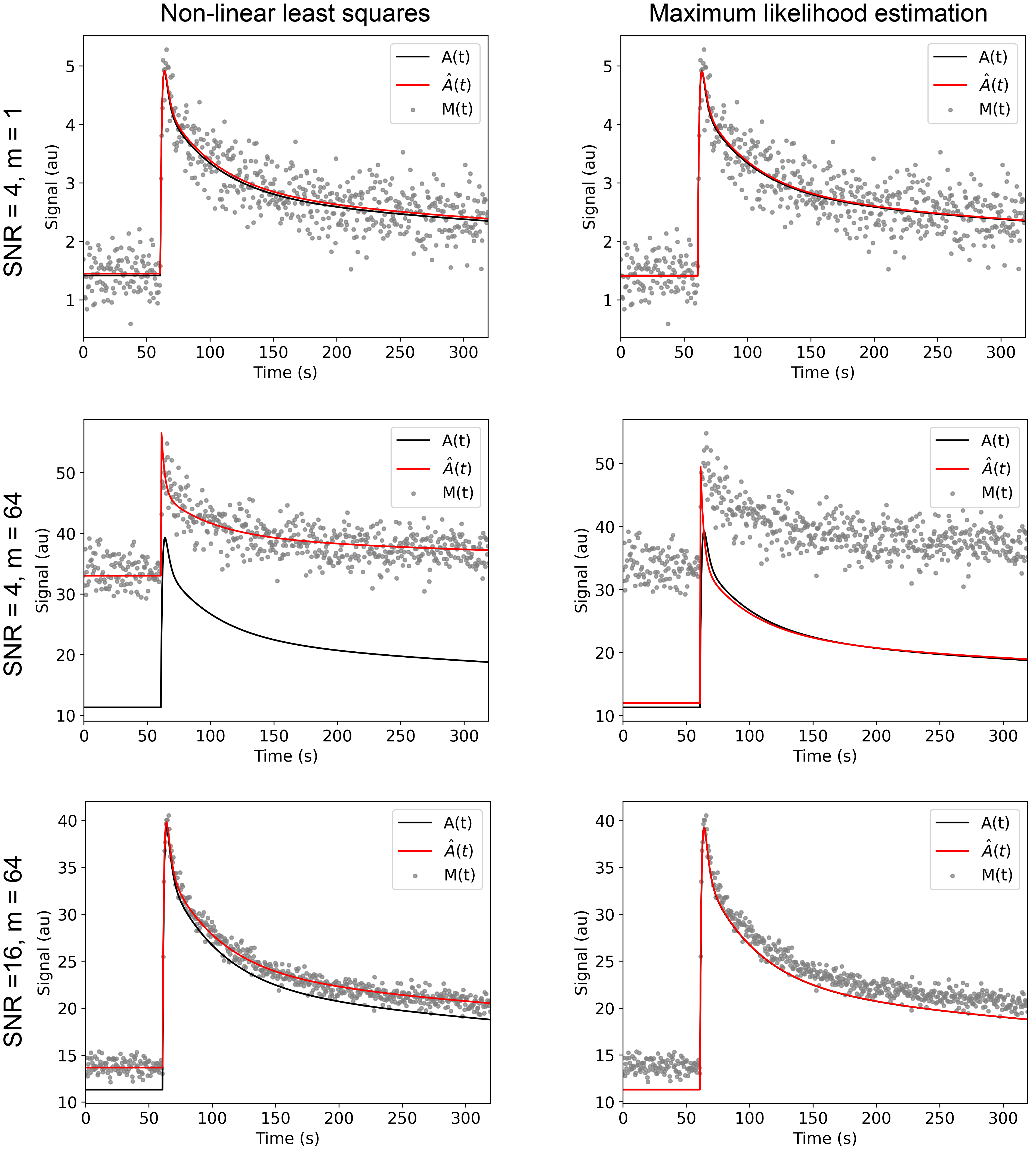
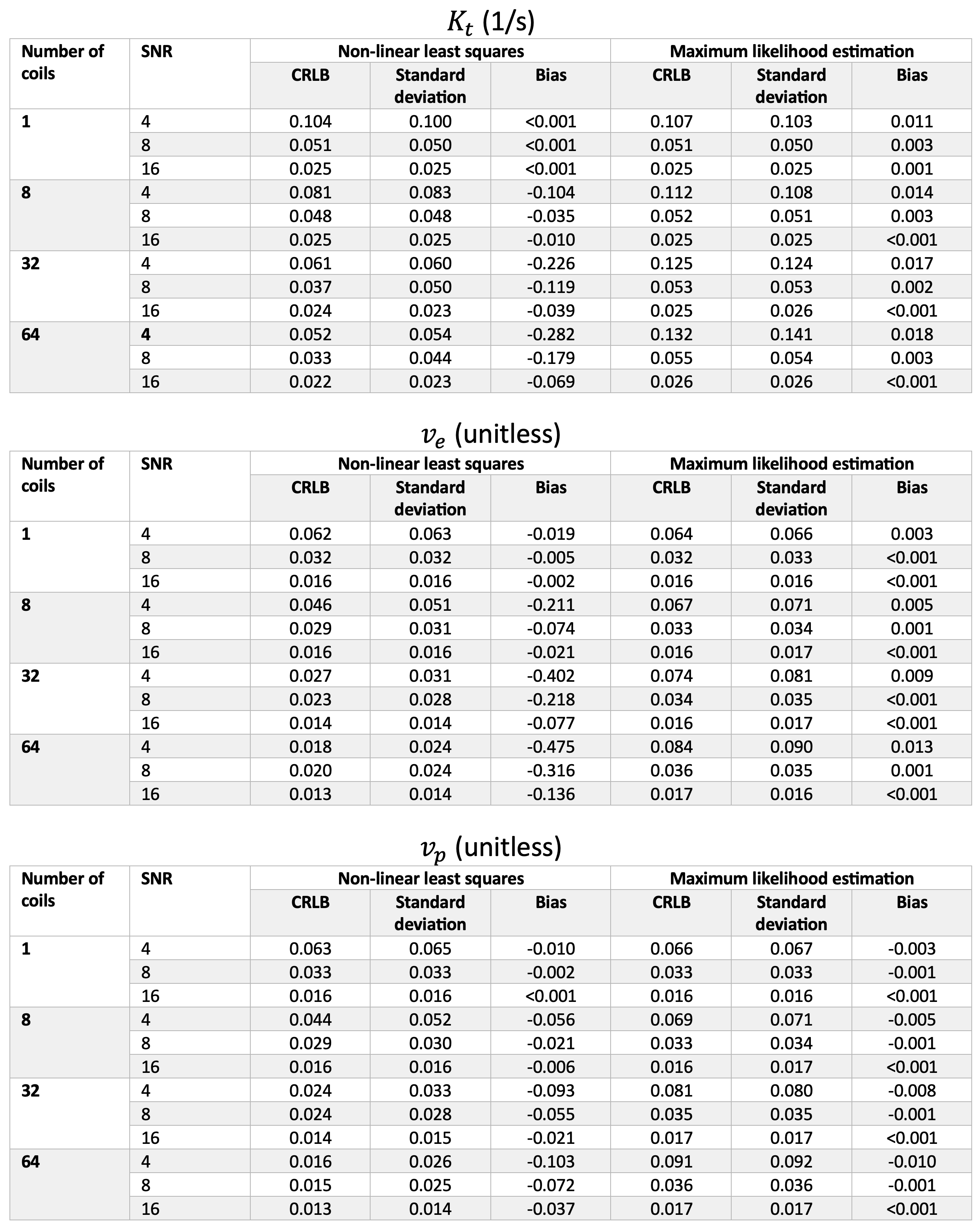
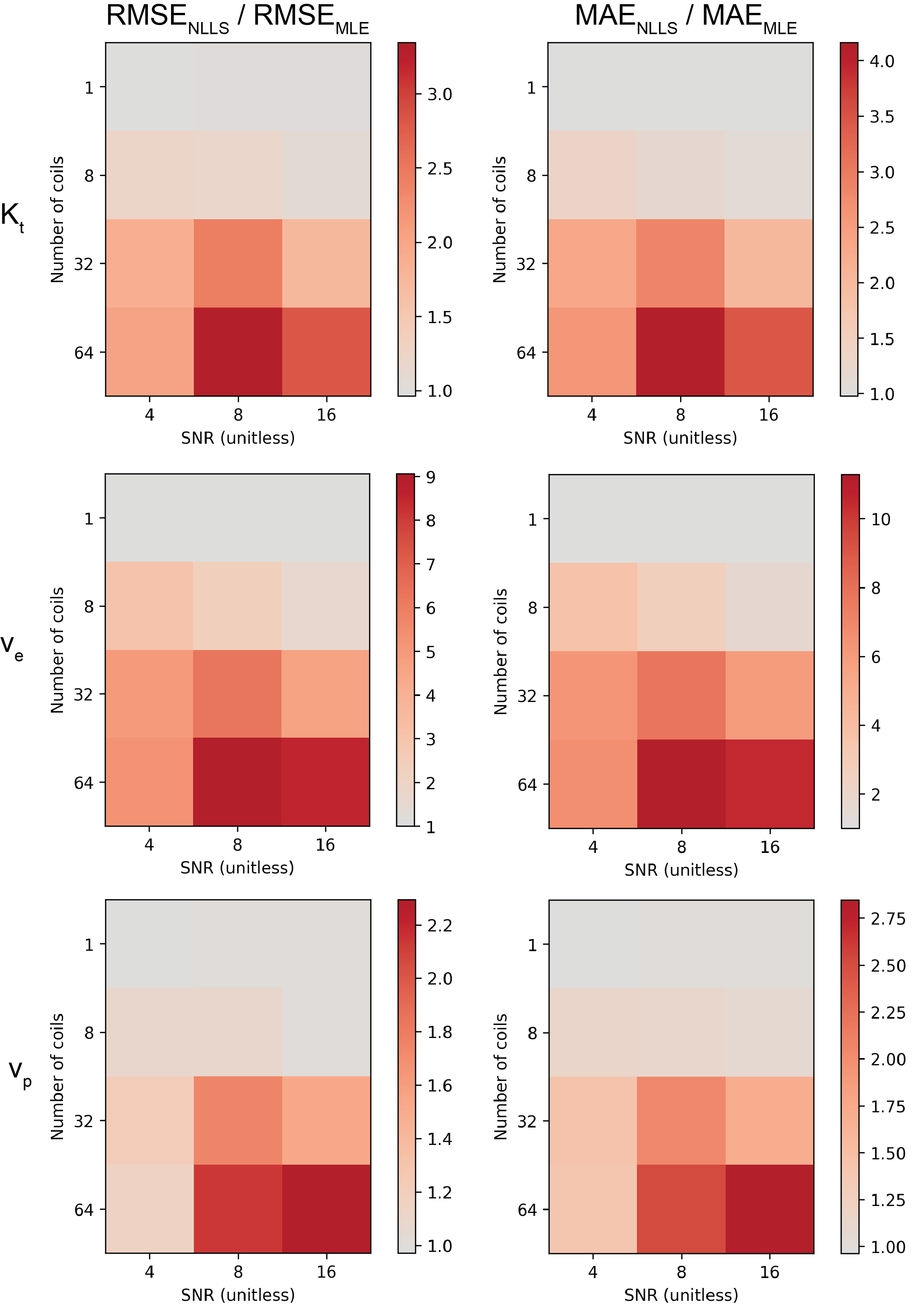
The NLLS method is increasingly biased as the number of coils increases and the SNR decreases (Table 1). The MLE method, however, has little bias across all SNR and coil combinations and which translates into reduced error for m ≥ 8 (Figure 3). Consistent with simulations for m = 1 the in vivo mouse pharmacokinetic kidney parameters estimated by MLE and NLLS were very similar (Figure 4).

Acknowledgements

Special thanks to Dr. Steven Sourbron for his valuable guidance.

References

1. Flouri, D., Lesnic, D. & Sourbron, S. P. Fitting the two-compartment model in DCE-MRI by linear inversion. Magn. Reson. Med. 76, 998–1006 (2016).

2. Fang, K. et al. Convolutional neural network for accelerating the computation of the extended Tofts model in dynamic contrast-enhanced magnetic resonance imaging. J. Magn. Reson. Imaging 53, 1898–1910 (2021).

3. Ulas, C. et al. Parameters: Application to stroke dynamic contrast-enhanced MRI. Front. Neurol. 10, 1–14 (2019).

4. Mittermeier, A., Ertl-Wagner, B., Ricke, J., Dietrich, O. & Ingrisch, M. Bayesian pharmacokinetic modeling of dynamic contrast-enhanced magnetic resonance imaging: Validation and application. Phys. Med. Biol. 64, (2019).

5. Fisher, R. On the mathematical foundations of theoretical statistics. Philos Trans R. Soc A 222, 309–368 (1922).

6. De Naeyer, D., De Deene, Y., Ceelen, W. P., Segers, P. & Verdonck, P. Precision analysis of kinetic modelling estimates in dynamic contrast enhanced MRI. Magn. Reson. Mater. Physics, Biol. Med. 24, 51–66 (2011).

7. Landheer, K. & Juchem, C. Are Cramér-Rao lower bounds an accurate estimate for standard deviations in in vivo magnetic resonance spectroscopy? NMR Biomed 34, e4521 (2021).

8. Blockley, N. P. et al. Field strength dependence of R1 and R2* relaxivities of human whole blood to ProHance, vasovist, and deoxyhemoglobin. Magn. Reson. Med. 60, 1313–1320 (2008).

9. Tofts, P. S. et al. Estimating kinetic parameters from dynamic contrast-enhanced T1- weighted MRI of a diffusable tracer: Standardized quantities and symbols. J. Magn. Reson. Imaging 10, 223–232 (1999).

10. Chen, H. et al. Extended graphical model for analysis of dynamic contrast-enhanced MRI. Magn. Reson. Med. 66, 868–878 (2011).

11. Sourbron, S. P., Michaely, H. J., Reiser, M. F. & Schoenberg, S. O. MRI-measurement of perfusion and glomerular filtration in the human kidney with a separable compartment model. Invest. Radiol. 43, 40–48 (2008).

12. Beeman, S. C. et al. Renal DCE-MRI Model Selection Using Bayesian Probability Theory. Tomography 1, 61–68 (2015).

13. Khalifa, F. et al. Models and methods for analyzing DCE-MRI: A review. Med. Phys. 41, (2014).

14. Tofts, P. & Kermode, A. Measurement of the blood-brain barrier permeability and leakage space using dynamic MR imaging. 1. Fundamental concepts. Magn Reson Med 17, 357–367 (1991).

15. Yang, C., Karczmar, G., Medved, M. & Stalder, W. Estimating the arterial input function using two reference tissues in dynamic contrast-enhanced MRI studies: Fundamental concepts and simulations. Magn Reson Med 52, 1110–1117 (2004).

16. Calamante, F. Arterial input function in perfusion MRI: A comprehensive review. Prog. Nucl. Magn. Reson. Spectrosc. 74, 1–32 (2013).

17. Bouhrara, M. & Spencer, R. G. Fisher Information and Cramer-Rao Lower Bound for Experimental Design in Parallel Imaging. Magn Reson Med 79, 3249–3255 (2018).

18. Wales, D. J. & Doye, J. Global Optimization by Basin-Hopping and the Lowest Energy Structures of Lennard-Jones Clusters Containing up to 110 Atoms. J Phys Chem A 101, 5111–5116 (1997).

19. Kay, S. M. Fundamentals of Statistical Signal Processing, Volume I Estimation Theory. (1993).

20. Matson, C. L. & Haji, L. Biased Cramér-Rao lower bound calculations for inequality-constrained estimators. J Opt Soc Am A Opt Image Sci Vis 23, 2702–2713 (2006).

21. Tukey, J. W. Exploratory Data Analysis. (1977).

22. Koay, C. G. & Basser, P. J. Analytically exact correction scheme for signal extraction from noisy magnitude MR signals. J. Magn. Reson. 179, 317–322 (2006).

Figures

Figure 1: Flow chart describing the generation of synthetic data. A) A measured arterial plasma concentration curve (grey circles) with its fit (red line, obtained via Equation 3); B) the tissue concentration curve calculated using Equation 2; C) The tissue signal curve calculated using Equation 1; D) the resulting synthetic signal after addition of noise sampled from a non-central χ distribution, which is the probability density function for sum-of-squares reconstructed phased-array MRI^17,22.

Figure 2: The generated synthetic signal without noise (black line), with noise (grey circles) and the estimated signal (red line) obtained using NLLS (left column) and MLE (right column) for three SNR and number of coils combinations. As the number of coils increases or SNR decreases the NLLS estimate becomes more biased since the noise becomes less accurately approximated by a Gaussian distribution. MLE incorporates such information, resulting in the estimated signal closer approximating the true signal.

Table 1: CRLBs and standard deviations obtained from NLLS and MLE for the three parameters $$$K_t$$$ (true value = 0.4 1/s), $$$v_e$$$ (true value = 0.6), and $$$v_p$$$ (true value = 0.1). For m ≥ 8 NLLS estimates are substantially biased, while for m = 1 both methods are nearly unbiased. Note that for some SNR and coil combinations the CRLBs for the NLLS estimates are substantially less than the CRLBs for the MLE estimates due to NLLS providing estimators with substantial bias.

Figure 3: RMSE from NLLS divided by the RMSE from MLE, first column; MAE from NLLS divided by MAE from MLE, second column. Kt, ve and vp are depicted in the first, second and third rows, respectively. For m ≥ 8 MLE substantially outperforms NLLS for both metrics (i.e., quantified errors from NLLS are greater errors from MLE, as depicted by shades of red). For m = 1 the two methods perform nearly identically (i.e., errors from both methods are nearly the same, as depicted by gray).

Figure 4: Pixel-wise estimates of the three pharmacokinetic parameters obtained with NLLS (left column) and MLE (right column) overlaid on top of the average over the entire DCE acquisition (grayscale). The sequence was a spoiled gradient echo with TE/TR = 1.2/6.5 ms, 600 repetitions, flip angle = 30°, imaging matrix = 100 x 100, field of view = 30 mm x 30 mm, received with a single quadrature coil. Consistent with simulation results for m = 1 the parameters estimated by NLLS and MLE are very similar.

Proc. Intl. Soc. Mag. Reson. Med. 32 (2024)

3123

DOI: https://doi.org/10.58530/2024/3123