3036
Highly under-sampled 3D Dynamic Hyperpolarized 13C Spiral Chemical Shift Imaging with Low Rank Plus Local Sparse Reconstruction1Diagnostic Radiology and Nuclear Medicine, University of Maryland, Baltimore, Baltimore, MD, United States
Synopsis
Keywords: Hyperpolarized MR (Non-Gas), Hyperpolarized MR (Non-Gas)
Motivation: Fully sampled 3DspCSI acquisition limits the temporal resolution for dynamic imaging
Goal(s): Our goal was to reconstruct highly under-sampled 3DspCSI without significant image artifacts
Approach: We proposed a low rank plus local sparse (LLS) reconstruction with two types of configurations to reconstruct the under-sampled 3DspCSI data
Results: proposed methods with both types of configurations can effectively reduce the image artifacts due to under-sampling. Type 2 configuration performs slightly better than Type 1 with less image artifacts due to the distinct patterns along the slice dimension
Impact: With the proposed LLS reconstruction, an effective acceleration of 4 can be achieved for 3DspCSI without significant image artifacts. The improvement in temporal resolution helps to quantify the metabolite kinetics during a fixed imaging window with hyperpolarized 13C agents
Introduction
3D Spiral Chemical Shift Imaging (3DspCSI) is an established metabolic imaging modality in various hyperpolarized (HP) 13C MRI applications1. Based on the 2DspCSI sequence, 3DspCSI acquires 4D k-space by applying phase encoding (PE) along the z-direction for each spiral interleaf. Due to hardware limitations, the acquisition time for one fully sampled 4D k-space is typically more than 10 seconds, insufficient temporal resolution for dynamic imaging. In previous study, we have developed customized Low Rank Plus Local Sparse(LLS) reconstruction for under-sampled 2DspCSI acquisitions with 3-fold effective acceleration2. In this study, we extend the LLS reconstruction to in vivo 3DspCSI with 4-fold acceleration.Method
Data acquisitionFor both digital simulation and in vivo scan, the 3DspCSI uses an 8-interleave 2D spiral trajectory with 40×40 mm FOV, 2.5×2.5 mm2 nominal in-plane resolution. 12 phase encoding steps are applied in slice direction with 48mm zFOV. 75% under-sampling is performed by pseudo-randomly selecting 2 out of 8 interleaves per PE step. TR of one under-sampled time point is 3 seconds. The pseudo-random selection table of the interleaves satisfies the condition that 4 adjacent under-sampled time points form a fully sampled block, which can be reconstructed at original temporal resolution (12 seconds/time point). A multiband RF excitation pulse3 was used for in vivo mouse imaging (1° on Pyr, 4° on Lac and Ala). A total of 16 under-sampled time points were acquired and used for image reconstruction.
Digital phantom simulation
A 3D dynamic phantom with cylinders representing the vasculature, kidneys, liver and heart in a mouse was created. Fully sampled data generates the ground truth (GT). Random Gaussian noise with the same scale as in vivo imaging was added to the retrospectively under-sampled data for simulation.
Experimental setup
In vivo imaging in a mouse was performed using clinical 3T GE MR scanner. A dose of 10 uL/g body weight of hyperpolarized pyruvate (~80 mM) was injected through a tail vein catheter.
Image reconstruction
Direct inversion of the encoding matrix using conjugate gradient on the under-sampled data gives the initial accelerated image (CGR4). Direct inversion on full k-space data combining the 4 adjacent time points gives the non-accelerated images (CGR1). Two types of configurations of the LLS reconstruction were tested for the simulation and applied to the in vivo data (Fig1). Type1 uses both slice and time dimension for low rank/sparse compression, whereas type2 only uses time dimension. Both types have 3 stages: global low rank in stage 1 and global low rank plus sparse in stage 2. In stage 3, low rank plus local sparse is applied to the blocked Casorati matrices. Type1 uses a block size of 1 along spectral dimension, while type2 uses a block size of 1 along both spectral and slice dimension.
Results and discussion
Fig2A-D presents GT of the digital phantom. Fig2E shows the simulation results at the selected slices and time points. Direct inverse on the 4-fold under-sampled data (CGR4) exhibit severe artifacts, while both types of LLS can successfully recover the ground truth images. In Fig2F-H, dynamic curves representing the mean intensities in the region of interest (ROI) taken from LLS recon results exhibit minor differences compared with ground truth. Fig3E-G displays results for the prospectively under-sampled in vivo acquisition reconstructed with CGR4 and two types of LLS. Artifacts seen in CGR4 recon are mostly eliminated through LLS recon. Meanwhile, LLS recon provides more dynamic information that indicates the time point when each metabolite reaches its peak, which cannot be captured through CGR1 recon. Without ground truth image, accuracy of LLS recon of the in vivo data is evaluated through comparing the average of 4 time points with corresponding CGR1 images, displayed in Fig4. In 4-point-average for type1 LLS, vasculature pyruvate has an artifact component contaminated by the high image intensity in the heart slice. Discrepancy is also observed in liver alanine slices. Image information in slices sharing distinct distributions could be interfered with each other as type1 LLS combines slice and time dimension for low rank/sparse compression. 4-point-average for type2 LLS shares high resemblance to the CGR1 images. Fig5A demonstrates the progressive reduction of artifacts through the three stages, whereas diminishing residual image illustrates the enforced consistency between reconstructed image and acquired data. Fig5B shows the effectiveness of artifact removal through LLS reconstruction, while type2 LLS performs slightly better than type1.Conclusion
With highly under-sampled data acquisition and LLS reconstruction, temporal resolution of 3DspCSI is enhanced from 5 frames/minute to 20 frames/minute without sacrificing spatial/spectral resolution. Type2 LLS is preferred over type1 LLS for image data with distinct spatial distribution along slice dimension.Acknowledgements
This work was supported by NIH grants R01 DK106395, R21 EB029083, and R21 DK131357 as well as DOD grants CA200996 and PR210572.References
[1] Josan S, Spielman D, Yen YF, Hurd R, Pfefferbaum A, Mayer D. Fast volumetric imaging of ethanol metabolism in rat liver with hyperpolarized [1-(13) C]pyruvate. NMR Biomed. 2012; 25(8):993-9.
[2] Zhu, et al. Improving temporal resolution in dynamic hyperpolarized 13C spiral chemical shift imaging using low rank plus local sparse reconstruction, Proc. Intl. Soc. Mag. Reson. Med. 29 (2023).
[3] Larson PE, Kerr AB, Chen AP, Lustig MS, Zierhut ML, Hu S, Cunningham CH, Pauly JM, Kurhanewicz J, Vigneron DB. Multiband excitation pulses for hyperpolarized 13C dynamic chemical-shift imaging. J Magn Reson. 2008 Sep;194(1):121-7.
Figures
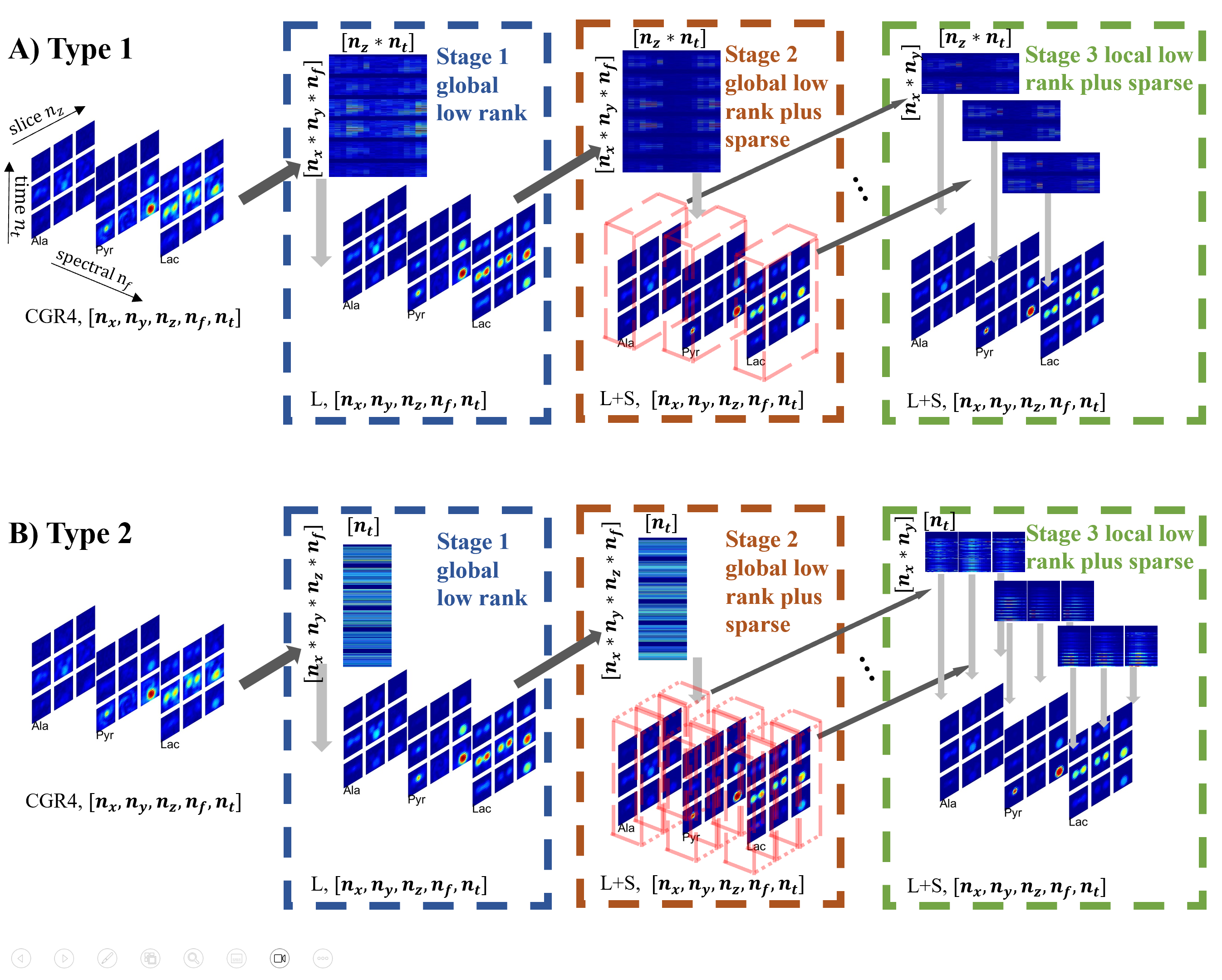
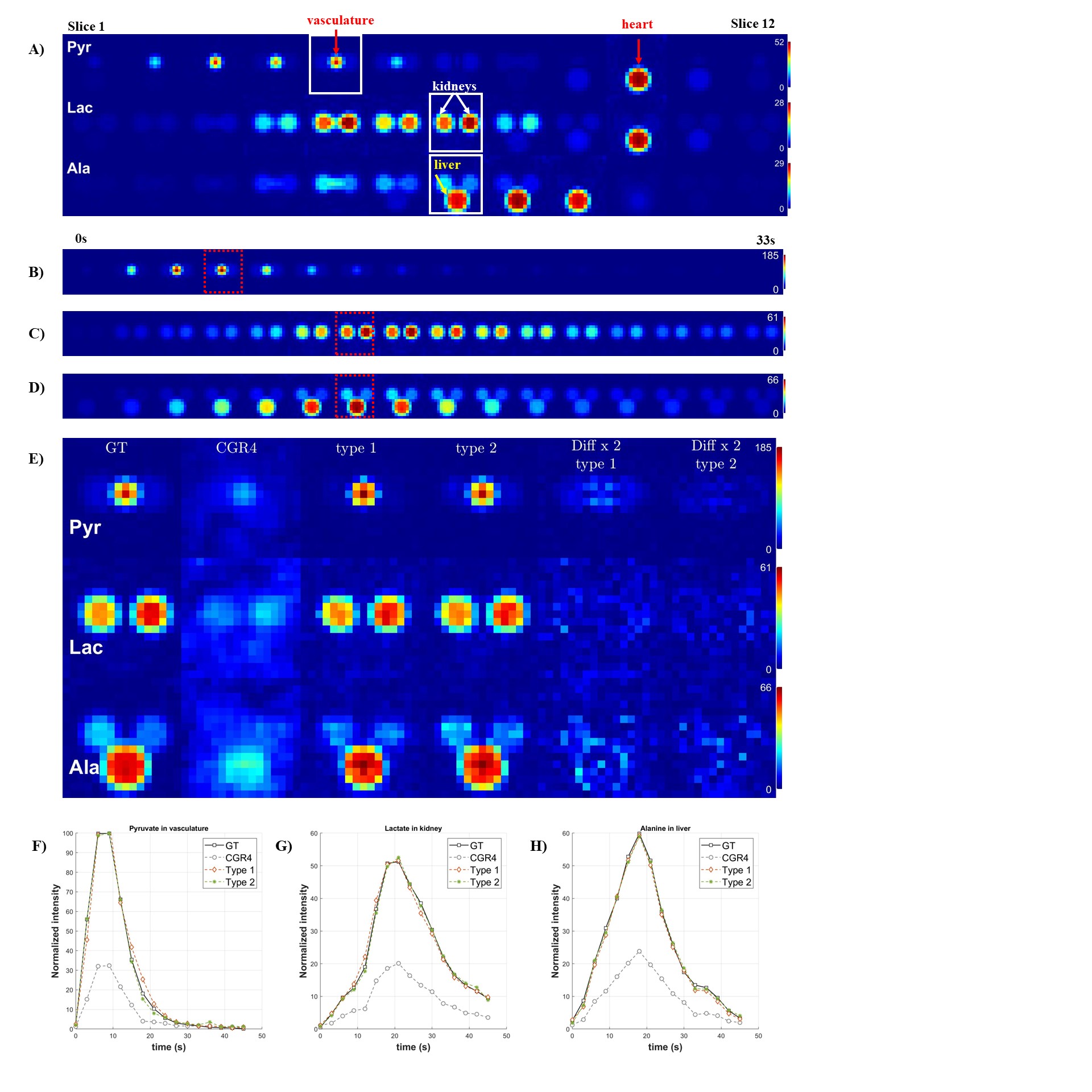
Figure 2. Simulation results from digital phantom.
2A: Time-averaged mean intensity of the ground truth (GT). Arrows point out the regions of interest (ROIs) where dynamic information is evaluated.
2B-D: Dynamic images of the ground truth (indicated by white squares in 2A)
2E: Reconstructed images with CGR4, type 1 LLS and type 2 LLS at the selected time point (indicated by red squares in 2B-D). Last two columns represent the difference between reconstructed images and GT.
2F-H: Dynamic curves representing mean intensities in the selected ROIs with respective reconstruction methods.
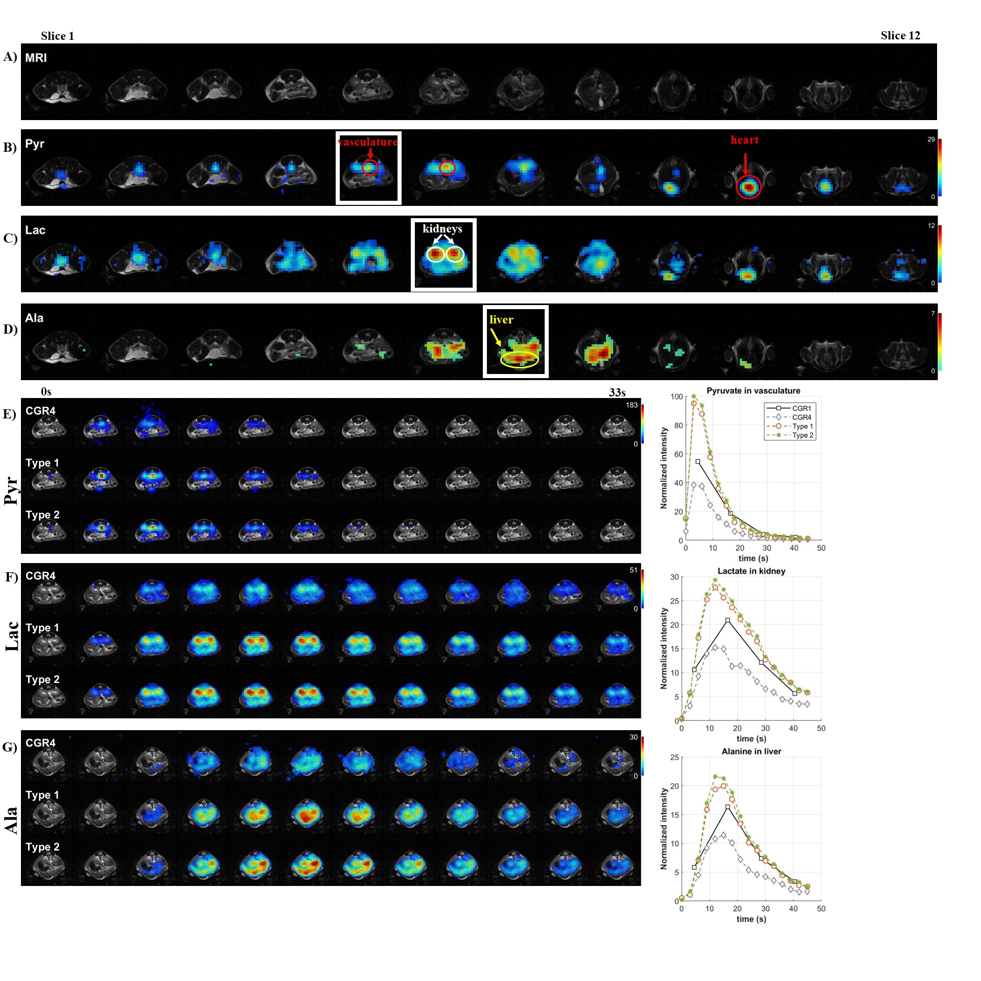
Figure 3. Reconstruction results for in vivo mouse imaging
3A: 1H MRI for anatomical overlay
3B-D: Time-averaged metabolic maps in all slices from reconstruction on the fully sampled k-space. Arrows point out ROIs.
3E-G: Accelerated (R=4) dynamic images at the representative slice. For each metabolite, 12 under-sampled time points starting at 0 seconds after start of data acquisition are presented. Dynamic curves of the non-accelerated images (CGR1) and accelerated images (CGR4, type1 LLS and type2 LLS) are plotted on the right.
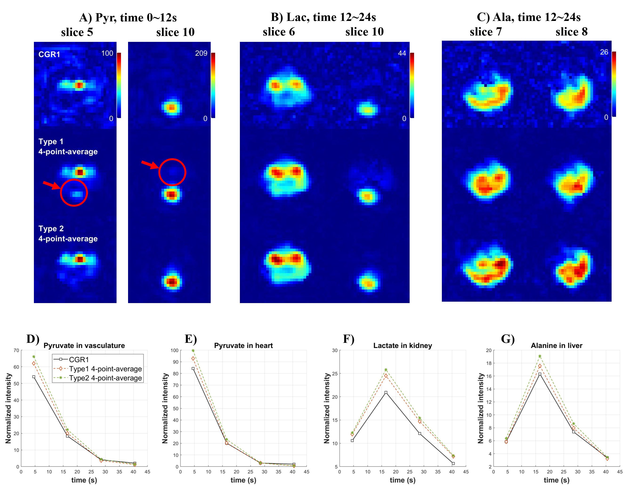
Figure 4. Non-accelerated (R=1) images from LLS reconstruction are generated through averaging 4 maps of spectra corresponding to a fully sampled block and compared to the CGR1 images to identify artifacts introduced during the LLS reconstruction.
4A: Slice 5 (vasculature) and slice 10 (heart) of the pyruvate images.
4B: Slice 6 (kidney) and slice 10 (heart) of the lactate images.
4C: Slice 7 (liver) and slice 8 of the alanine images.
4D-G: Dynamic curves for the non-accelerated images of the corresponding ROIs.
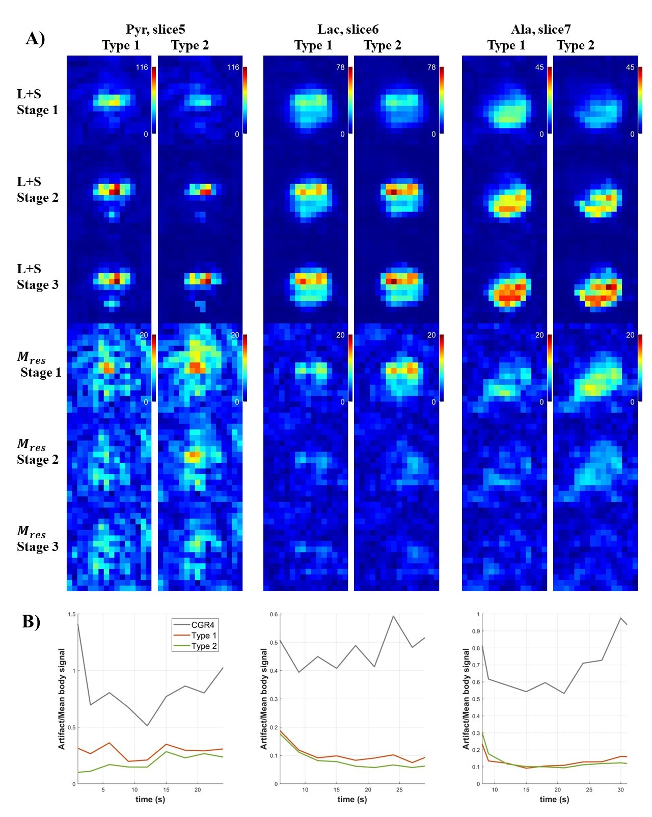
Figure 5
5A: Row 1 - 3: Magnitude of the peak frequency bin in L+S image at selected slice and time point after each stage of LLS reconstruction.Row 4 - 6: Corresponding residual image representing inconsistency between reconstructed L+S image and acquired data after each stage of LLS reconstruction
5B: Artifacts to mean body signal ratio at the specific slice and time point is characterized by mean intensity outside the mouse body, normalized to the mean signal inside the body. Ratios are plotted in selected time window where there is sufficient SNR to quantify the mean body signal.