3034
Integrated B0 and B1 mapping and image correction for hyperpolarized Carbon-13 metabolic imaging in the human brain1Oxford Centre for Clinical Magnetic Resonance Research (OCMR), University of Oxford, Oxford, United Kingdom, 2Department of Oncology, University of Oxford, Oxford, United Kingdom, 3Department of Radiology, Oxford University Hospitals, Oxford, United Kingdom, 4Department of Physiology, Anatomy and Genetics, University of Oxford, Oxford, United Kingdom, 5GE HealthCare, Munich, Germany, 6Alma Mater Studorium, University of Bologna, Bologna, Italy
Synopsis
Keywords: Hyperpolarized MR (Non-Gas), Hyperpolarized MR (Non-Gas), B1 correction, B0 correction
Motivation: B0 and B1 inhomogeneities affect signal quantification and kinetic modelling but are challenging to map and correct for in hyperpolarized MRI due to the signal being exogenous and non-renewable.
Goal(s): Develop a fully-integrated B0 and B1 mapping method that does not require specialized pulse sequence programming, additional hardware, nor any additional carbon-13 dose.
Approach: Varying echo times and flip angles in the imaging sequence.
Results: The in-vivo field maps agreed well with independently acquired maps and could correct for B0 off-resonance blurring and B1 inhomogeneity.
Impact: A fully-integrated B0 and B1 mapping and correction method for hyperpolarized carbon-13 MRI is presented and validated in vivo. This method is readily implemented and can improve image quality, helping 13C metabolic imaging become more robust for clinical studies.
Introduction
Hyperpolarized carbon-13 metabolic imaging is an emerging technique whereby metabolic processes can be probed by imaging carbon-13 labelled molecules and their conversion into downstream metabolites [1,2], enabling the early monitoring of various diseases before detectable structural changes [3-5]. Correcting for field inhomogeneities in hyperpolarized MRI has been a challenge due to the exogenous and non-renewable nature of the hyperpolarized signal. Currently, few B0 and B1 mapping methods for hyperpolarized MRI carbon-13 MRI exist that do not require additional coils or phantoms [6,7], specialized pulse sequence programming software [8], or the administration of an additional hyperpolarized carbon-13 dose. This means that coil-induced inhomogeneities and off-resonance blurring artifacts are often not adequately corrected for, affecting signal quantification and kinetic modelling [9,10]. We propose a simple method to integrate B0 and B1 mapping into a hyperpolarized carbon-13 imaging sequence, using varied flip angle (FA) and varied echo time (TE) repetitions of a standard pulse sequence. We validate, in 2 human brain scans, the acquisition of inherently co-registered B0 and B1 maps within the imaging sequence. Furthermore, we demonstrate using the acquired field maps to correct for inhomogeneities and off-resonance blurring.Methods
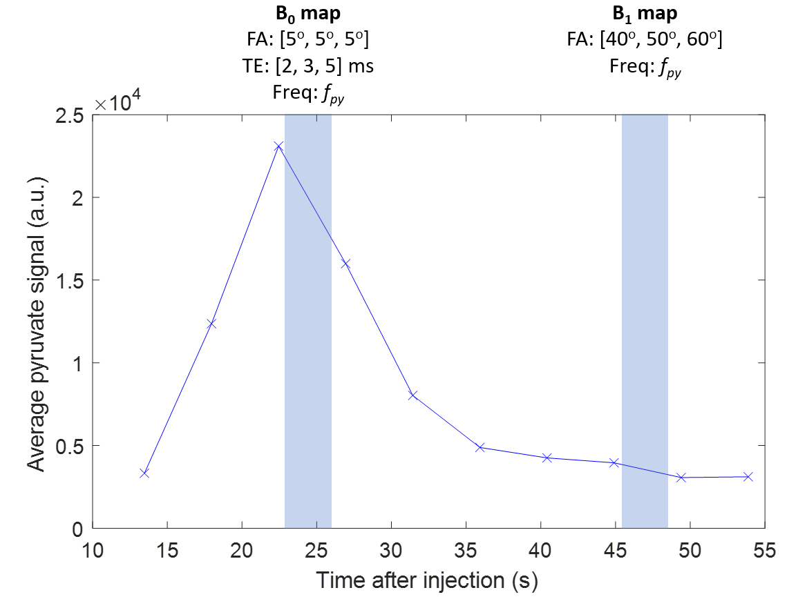
The study was conducted after local ethical approval and written informed consent from participants. Images were acquired on a 3T GE Premier (GE Healthcare, WI) using a dual-tuned 1H/13C birdcage head coil (Rapid Biomedical, Germany). Two healthy volunteers (male; age 64 and 67) were scanned after intravenous injection of 0.4ml/kg of 250mM hyperpolarized sodium [1-13C]pyruvate following polarization for ~4hours in a SPINLab hyperpolarizer (GE Healthcare, WI) [11]. Transmit gain (TG) for 13C was calibrated using a thermal 13C urea phantom placed by the participant’s head. The imaging protocol used a spectral-spatial multi-slice single-arm spiral sequence (16x16 acquisition matrix, 240x240mm FOV, eight 20mm slices, 32x32 reconstruction matrix) [12] with pyruvate (FApy:5o), lactate (FAlac:15o), and bicarbonate (FAbic:60o) maps acquired at ~4s intervals.Variable TE acquisitions (2, 3, and 5 milliseconds) at the pyruvate frequency were interleaved ~20s after injection using low flip angles (5o) (Fig. 1). The B0 map was obtained by fitting the signal phase using the MEDI toolbox [13-15], and evaluated against a standard proton B0 map acquired using the same coil.
Variable FA acquisitions (40o, 50o, and 60o) at the pyruvate frequency were interleaved ~45s after injection for B1 mapping. The signal was fitted voxel-wise to the following equation:
$$S=M_0{\cdot}exp\left(-\frac{TR}{T_1}\right)^{TR{\cdot}Time_t}{\cdot}sin(\Delta{B_1}{\cdot}FA_{Time})\prod_{Time_0}^{Time_t}cos(\Delta{B_1}{\cdot}FA_{Time})$$
where S is the signal, M0 is initial magnetization, TR is repetition time, FA is flip angle, Time is a vector of time points during acquisition, and ΔB1 is transmit B1 variation.
The in vivo B1 map was evaluated against a separately acquired B1 Map using a spherical silicone-oil phantom (2D CSI, 1.4ms partial self-refocused pulse, 16x16 acquisition matrix, 240x240mm FOV, 8.3s TR, FAs=40,60,80,90,100,120,160o, signals fitted voxel-wise to $$$S=M_0{\cdot}sin(\Delta B_1{\cdot}FA_{Time})$$$).
Image correction was performed after smoothing of both field maps using polynomial fitting and extrapolation (second order, kernel width = 4) [16]. Multi-frequency interpolation (MFI) was used for B0 correction [17,18]. Prior to B1 correction, metabolite maps were divided by $$$sin(FA_{metabolite})$$$. Assuming transmit-receive reciprocity, B1 correction was then performed:
$$I'_{metabolite}=I{\cdot}\frac{sin(FA_{metabolite})}{sin(\Delta{B_1}{\cdot}FA_{metabolite})}{\cdot}\frac{1}{\Delta{B_1}}$$
Where I’ is corrected image and I is measured image.
Results
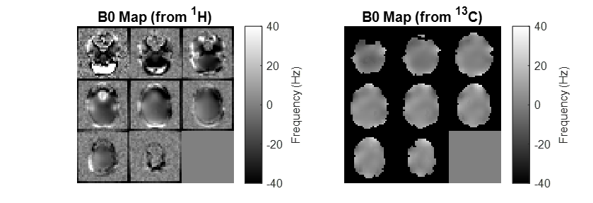
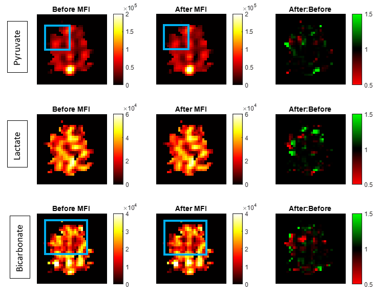
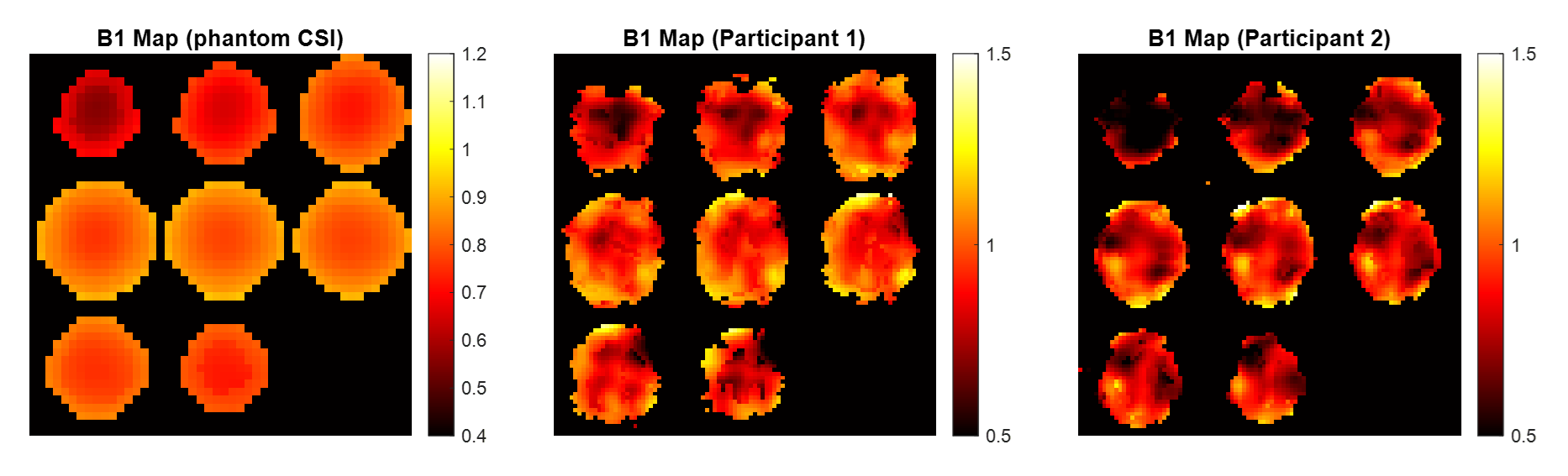
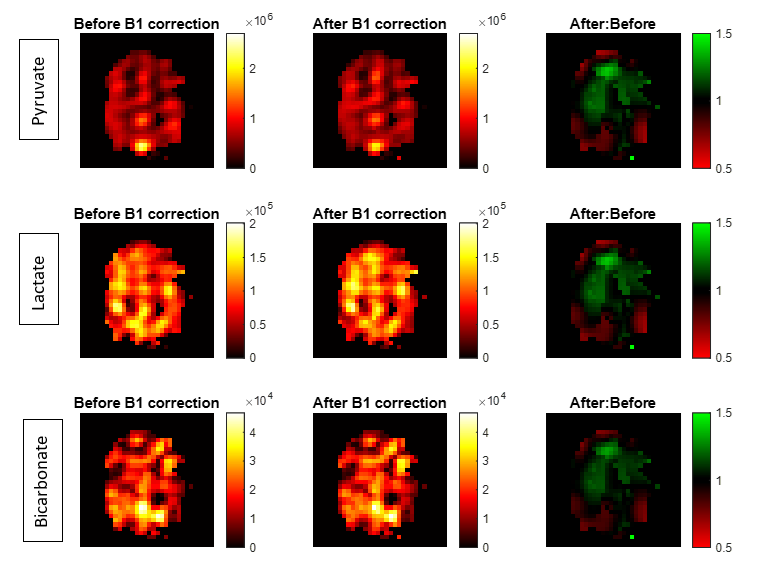
B0 maps from 13C imaging sequence match well with proton B0 maps (standard deviations: 14.04 Hz from 13C and 17.78 Hz from 1H (Participant 1); 22.43 Hz from 13C and 26.78 Hz from 1H (Participant 2)) (Fig. 2). Applying MFI shows deblurring in the metabolite maps (Fig. 3). In vivo 13C ΔB1 maps (mean ΔB1 ± SD: 0.98±0.11 (Participant 1); 0.92±0.12 (Participant 2)) show good agreement with the phantom B1 Map (Fig. 4). B1 correction increases signal intensity towards the coil center (Fig. 5). The average signal change is -0.14%±3.77%.Discussion
This study validated a fully-integrated B0 and B1 mapping method which is more straightforward to implement than existing methods, only requiring altering the parameters FA, TE, and TR of a standard pulse sequence. The acquired maps are inherently co-registered and patient-specific. The B0 map was acquired roughly around the middle of the bolus to maximize SNR and the B1 map was acquired with high flip-angles at the end of pyruvate bolus to effectively use up residual magnetization. Field homogeneities are assumed to be similar for all metabolites of interest.Conclusion
A B0 and B1 mapping method which is fully integrated into the carbon-13 imaging sequence is presented and validated in vivo for two human brains, and shows good agreement with independently acquired field maps. B0 and B1 correction shows sharpened images and improved signal homogeneity.Acknowledgements
This work was supported by the John Fell Fund. Acknowledgement must also be given to Oxford-MRC Doctoral Training Partnership iCASE award, the Oxford-Radcliffe Scholarship, and GE HealthCare for funding this project.References
[1] M. Vaeggemose, R. F. Schulte, and C. Laustsen, ‘Comprehensive Literature Review of Hyperpolarized Carbon-13 MRI: The Road to Clinical Application’, Metabolites, vol. 11, no. 4, p. 219, Apr. 2021, doi: 10.3390/metabo11040219.
[2] P. E. Z. Larson and J. W. Gordon, ‘Hyperpolarized Metabolic MRI—Acquisition, Reconstruction, and Analysis Methods’, Metabolites, vol. 11, no. 6, Art. no. 6, Jun. 2021, doi: 10.3390/metabo11060386.
[3] M. A. Schroeder, L. E. Cochlin, L. C. Heather, K. Clarke, G. K. Radda, and D. J. Tyler, ‘In vivo assessment of pyruvate dehydrogenase flux in the heart using hyperpolarized carbon-13 magnetic resonance’, Proc. Natl. Acad. Sci., vol. 105, no. 33, pp. 12051–12056, Aug. 2008, doi: 10.1073/pnas.0805953105.
[4] Z. Ye, B. Song, P. M. Lee, M. A. Ohliger, and C. Laustsen, ‘Hyperpolarized carbon 13 MRI in liver diseases: Recent advances and future opportunities’, Liver Int., vol. 42, no. 5, pp. 973–983, May 2022, doi: 10.1111/liv.15222.
[5] R. Woitek et al., ‘Hyperpolarized Carbon-13 MRI for Early Response Assessment of Neoadjuvant Chemotherapy in Breast Cancer Patients’, Cancer Res., vol. 81, no. 23, pp. 6004–6017, Dec. 2021, doi: 10.1158/0008-5472.CAN-21-1499.
[6] I. Park et al., ‘Development of methods and feasibility of using hyperpolarized carbon-13 imaging data for evaluating brain metabolism in patient studies’, Magn. Reson. Med., vol. 80, no. 3, pp. 864–873, 2018, doi: 10.1002/mrm.27077.
[7] P. M. Lee et al., ‘Whole-Abdomen Metabolic Imaging of Healthy Volunteers Using Hyperpolarized [1-13C]pyruvate MRI’, J. Magn. Reson. Imaging, vol. 56, no. 6, pp. 1792–1806, 2022, doi: 10.1002/jmri.28196.
[8] S. Tang et al., ‘A regional bolus tracking and real-time B1 calibration method for hyperpolarized 13C MRI’, Magn. Reson. Med., vol. 81, no. 2, pp. 839–851, 2019, doi: 10.1002/mrm.27391.
[9] D. Mammoli et al., ‘Kinetic Modeling of Hyperpolarized Carbon-13 Pyruvate Metabolism in the Human Brain’, IEEE Trans. Med. Imaging, vol. 39, no. 2, pp. 320–327, Feb. 2020, doi: 10.1109/TMI.2019.2926437.
[10] B. T. Chung et al., ‘Hyperpolarized [2–13C]pyruvate MR molecular imaging with whole brain coverage’, NeuroImage, vol. 280, p. 120350, Oct. 2023, doi: 10.1016/j.neuroimage.2023.120350.
[11] J. T. Grist et al., ‘Quantifying normal human brain metabolism using hyperpolarized [1–13C]pyruvate and magnetic resonance imaging’, NeuroImage, vol. 189, pp. 171–179, Apr. 2019, doi: 10.1016/j.neuroimage.2019.01.027.
[12] R. F. Schulte et al., ‘Saturation-recovery metabolic-exchange rate imaging with hyperpolarized [1-13C] pyruvate using spectral-spatial excitation’, Magn. Reson. Med., vol. 69, no. 5, pp. 1209–1216, 2013, doi: 10.1002/mrm.24353.
[13] T. Liu, C. Wisnieff, M. Lou, W. Chen, P. Spincemaille, and Y. Wang, ‘Nonlinear formulation of the magnetic field to source relationship for robust quantitative susceptibility mapping’, Magn. Reson. Med., vol. 69, no. 2, pp. 467–476, 2013, doi: 10.1002/mrm.24272.
[14] B. Kressler, L. de Rochefort, T. Liu, P. Spincemaille, Q. Jiang, and Y. Wang, ‘Nonlinear Regularization for Per Voxel Estimation of Magnetic Susceptibility Distributions From MRI Field Maps’, IEEE Trans. Med. Imaging, vol. 29, no. 2, pp. 273–281, Feb. 2010, doi: 10.1109/TMI.2009.2023787.
[15] L. de Rochefort, R. Brown, M. R. Prince, and Y. Wang, ‘Quantitative MR susceptibility mapping using piece-wise constant regularized inversion of the magnetic field’, Magn. Reson. Med., vol. 60, no. 4, pp. 1003–1009, 2008, doi: 10.1002/mrm.21710.
[16] K. P. Pruessmann, M. Weiger, M. B. Scheidegger, and P. Boesiger, ‘SENSE: Sensitivity encoding for fast MRI’, Magn. Reson. Med., vol. 42, no. 5, pp. 952–962, 1999, doi: 10.1002/(SICI)1522-2594(199911)42:5<952::AID-MRM16>3.0.CO;2-S.
[17] L.-C. Man, J. M. Pauly, and A. Macovski, ‘Multifrequency interpolation for fast off-resonance correction’, Magn. Reson. Med., vol. 37, no. 5, pp. 785–792, 1997, doi: 10.1002/mrm.1910370523.
[18] A. Nylund, ‘Off-resonance correction for magnetic resonance imaging with spiral trajectories’, Bachelor of Science Thesis, KTH Royal Institute of Technology, Sweden, 2014. Accessed: Nov. 01, 2023. [Online]. Available: https://www.semanticscholar.org/paper/Off-resonance-correction-for-magnetic-resonance-Nylund/f2986a42d2bc22aa58ab0a555a5268e8c7b0dc2b
Figures