3007

Field Camera input to Virtual Phantom (ViP) scanner acquisitions for quality assurance of derived MRI quantities: First Proof-of-Principle.

Peter Gatehouse¹, Andrew Scott¹, Gaby Captur², Muhammad Usman¹, Ronald Mooiweer¹, Dudley Pennell¹, and Sonia Nielles-Vallespin¹
¹Cardiovascular MR, Royal Brompton Hospital, London, United Kingdom, ²University College London, London, United Kingdom

Synopsis

Keywords: Phantoms, New Devices, Precision & Accuracy, Field Camera, Virtual Phantom

Motivation: Quality assurance (QA) of quantities derived from MRI requires elaborate phantoms. Instead, we send modulated RF signals into the scanner representing any initial test object (previous “Virtual Phantom ViP”) avoiding physical phantom difficulties.

Goal(s): Proof-of-principle of a novel step for QA of derived quantities, by combining two previous methods: a Field Camera (FC) to govern ViP.

Approach: QA compares outputs from the unmodified scanner against the initial object. Tests evaluated the prototype technically, plus a derived QA example: myocardial bloodflow by first-pass contrast-enhanced myocardial perfusion.

Results: Phase stability without phase-locking to scanner was marginal, while first demonstrating FC+ViP QA of a derived quantity.

Impact: Quality assurance of derived quantities can require elaborate physical phantoms. Instead, we demonstrate novel field camera governance of the unmodified scanner's virtual phantom acquisition, reconstruction and analysis. We call for vendor cooperation in a new standardised inexpensive quality control interface.

Introduction

Quality assurance (QA) of quantities derived from MRI currently requires elaborate phantoms as reference standards^1-7. There is an unsolved need regarding practical difficulties of some physical phantoms especially for intersite or intervendor work. Alternatively, previous work has transmitted modulated RF signals into the scanner (“Virtual Phantom ViP”)^8-11 with controlled modulations for any required physics, representing the Simulated Test Object (STO) “input”, to be compared with the scanner “output” to achieve the QA purpose. This work aims for proof-of-principle of a novel step in capability for QA of derived quantities by combining two prior methods, using a prototype Field Camera (FC)^12-15 to govern ViP (FC+ViP, named Ariel¹⁶).

Methods

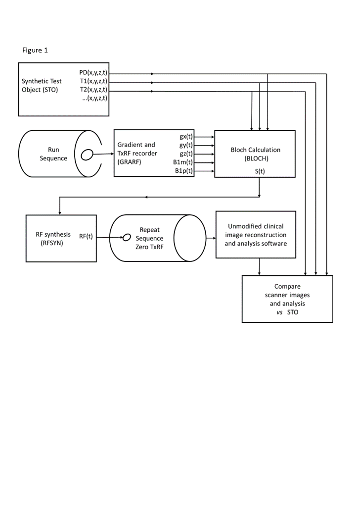
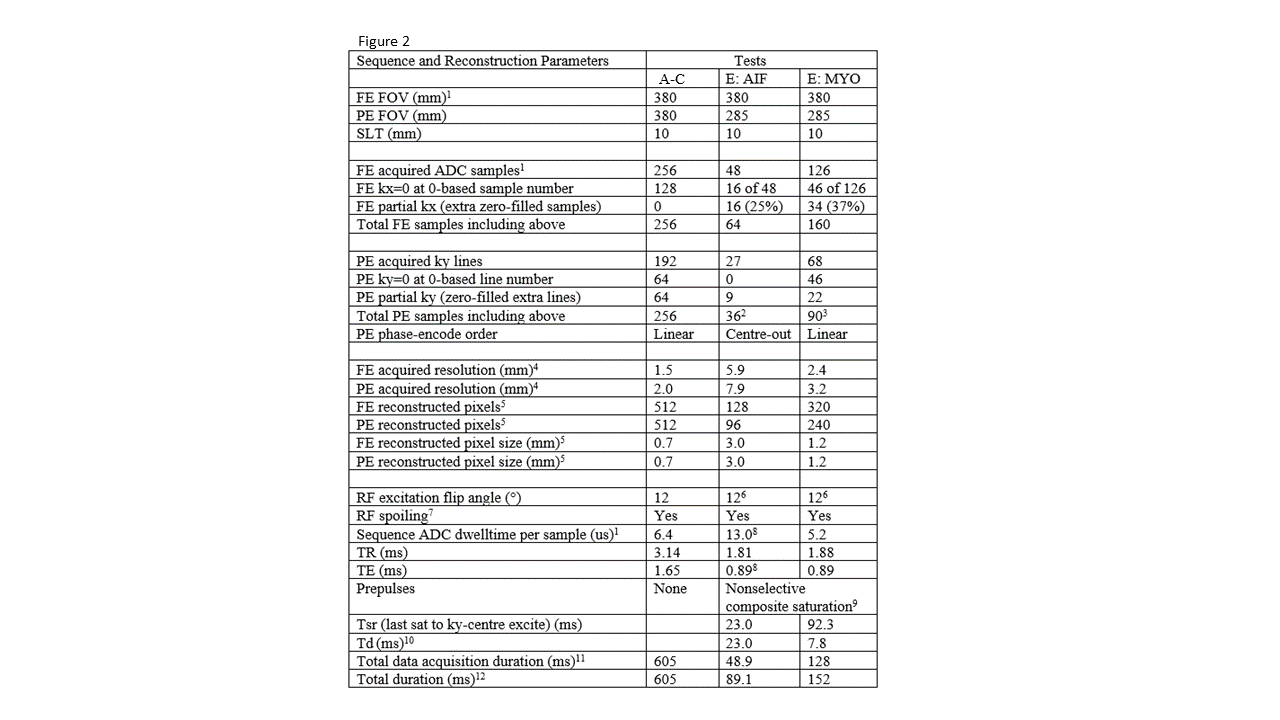
Like ViP, Ariel starts with the STO modeling the quantity where QA is required (Figure 1). Using the FC to record the entire pulse sequence, Ariel calculates by Bloch computation¹⁷ the continuous RF signal that would be emitted by the physical version of the STO during the sequence. Ariel transmits this calculated RF signal for reception, reconstruction and any further parametric derivations as normally performed by the scanner and further analysis programs used routinely. The analysis output is compared to the input STO for QA. Ariel operates continuously during the pulse sequence, after one initial trigger to synchronise with the scanner. Images were received by an unmodified scanner (3T Vida, Siemens Healthineers, “4-channel Flex Coil, small” around the Ariel Tx loop), reconstructed as sum-of-squares magnitude, without gradient nonlinearity correction nor other filtering. For nutation during BLOCH, the GRARF B1 amplitude was calibrated using the flip angles and Mz. A conventional phantom enabled the usual scanner prescan “adjustments”.
Tests A-C (parameters, Figure 2) using STO T1=200ms T2=20ms conducted basic technical evaluation of the prototype, i.e. these are not proposed QA applications.
Test A: Fidelity of GRARF and FE Rolloff: STO = square of uniform PD, T1 and T2, side 285mm. A total of 30 Ariel scans investigated PE ghosting and GRARF recordings.
Test B: PSFs and long-term phase stability: STO = 9 points (2.2x3.0mm FExPE) distributed obliquely over FOV, repeated for 60’.
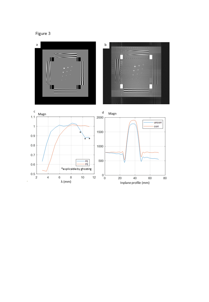
Test C: Resolution and Slice-profile (see Figure 3).
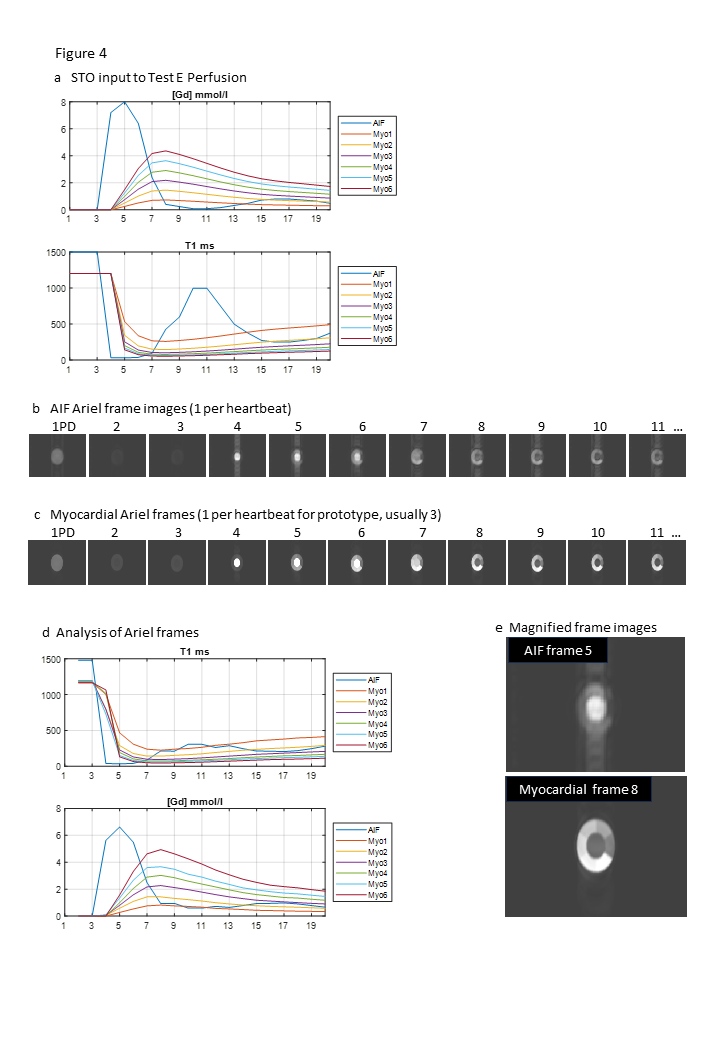
Test E (parameters, Figure 2) is the main aim, applying Ariel to QA a derived quantity (Figure 4): for example, derivation of myocardial blood flow (MBF) from first-pass contrast-enhanced (GBCA) perfusion¹⁸; MBF is clinically interesting and requires QA⁴.

Results

Test A: Phase-encode ghosting was consistent for repeated scans. It changed for each GRARF recording, and reduced slightly using 5-averaged GRARF. FE magnitude rolled off consistently across all Test A-D images (symmetrically to 58% at ±141mm).
Test B: PSF FWHM along FE was reliable, but PE FWHM of offset points reached 6.7mm. Over 60’ the PE FOV drifted 1.5cm monotonically.
Test C: (Figure 3): Phase-encode resolution was again compromised, while slice-profile was reasonable after correcting for FE rolloff.
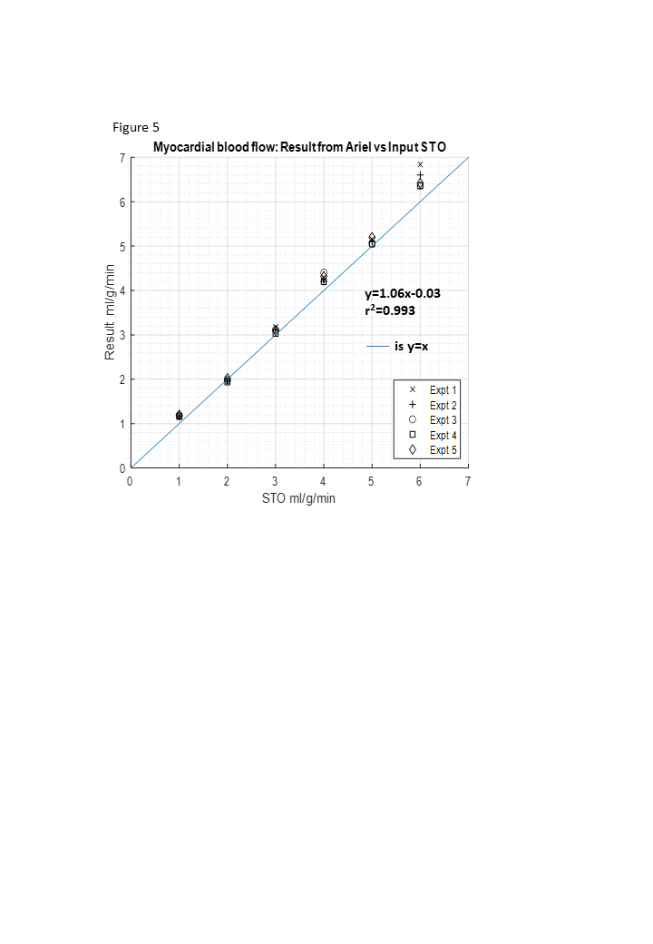
Test E: The magnitude, calculated T1¹⁹, hence [GBCA] of each frame (Figure 4d) enabled deconvolution analysis for MBF showing reproducible prototype agreement with the input STO values of each myocardial segment (Figure 5).

Discussion

While Test E perfusion MBF agreement vindicated Ariel’s aim, limitations are noted: For this prototype, deconvolution analysis for Test E was locally written in Matlab, but should usually evaluate all the software used clinically. Frequency-encode rolloff was associated with slow prototype microcontroller RFSYN timepoints (6.4us), not the AD9914 IC used. Phase-encode ghosting, degrading PE resolution, arose from imperfect GRARF recordings, not OCXO instability. However, temporal phase stability was borderline; complicated k-space sampling or long scans would demand phase-locked scanner and Ariel clocks. The OCXO of RFSYN was free-running because Ariel required no connections other than the standard fibre-optic trigger output of the scanner. The original notion of Ariel would calculate and transmit in real-time, even calibrating the scanner “tuning” adjustments; perhaps feasible²⁰but beyond the prototype's design. Further, the GRARF imperfections required correction work. Scanner Larmor frequency modulation was observed (perhaps “B0 shift compensation”) which fortunately cancelled out. Multiple/multiplexed RFSYN into separate loops distributed across the PE direction could support parallel imaging.

Conclusions

For the QA aim, Ariel extended ViP by combining it with a prototype field camera and continuous operation, needing no prior knowledge of sequence or ADC timings, k-space ordering, accelerations nor reconstruction strategies (ML might require realistic STO images^21,22).
The extra electronics of Ariel, particularly GRARF, might be eliminated²³: we propose²⁴ that a simple inexpensive ‘interface’ for QA (cf. automotive OBD2), might be standardised among MRI vendors, to eliminate GRARF (by far the hardest work of Ariel). With little extra hardware, “built-in” standardised QA of derived quantities could be openly available for all MR.

Acknowledgements

The Ariel idea occurred during initial discussion of the myocardial T1 test phantom (T1MES) with the cardiovascular MRI research group of Professor James Moon, then at the National Heart Hospital London.

References

1 Cashmore MT, McCann AJ, Wastling SJ et al. Clinical quantitative MRI and the need for metrology (2021). Br J Radiol 94: 20201215

2 Keenan KE, Ainslie M, Barker AJ et al. Quantitative magnetic resonance imaging phantoms: a review and the need for a system phantom (2018). Magn Res Med 79:48-61.

3 Captur G, Gatehouse P, Keenan KE et al. A medical device-grade T1 and ECV phantom for global T1 mapping quality assurance—the T1 Mapping and ECV Standardization in cardiovascular magnetic resonance (T1MES) program (2016). JCMR 18:58

4 Chiribiri A, Schuster A, Ishida M et al. Perfusion Phantom: An Efficient and Reproducible Method to Simulate Myocardial First-Pass Perfusion Measurements with Cardiovascular Magnetic Resonance (2013). Magn Res Med 69:698-707.

5 Stupic KF, Ainslie M, Boss MA et al. A standard system phantom for magnetic resonance imaging (2021). Magn Res Med 86:1194-1211.

6 Gadda G, Cocozza S, Gambaccini M et al. NO-HYPE: a novel hydrodynamic phantom for the evaluation of MRI flow measurements (2021). Med and Biol Eng and Comput 59:1889-1899.

7 Swailes NE, MacDonald ME, Frayne R. Dynamic phantom with heart, lung and blood motion for initial validation of MRI techniques (2011). JMRI 34:941-6.

8 Saint-Jalmes H, Eliat P, Bezy-Wendling J et al. ViP MRI: virtual phantom magnetic resonance imaging (2014). Magn Reson Mater Phy 27:419-24.

9 Salvati R, Hitti E, Bellanger J-J et al. Fat ViP MRI: Virtual Phantom Magnetic Resonance Imaging of water-fat systems (2015). MRI 2015. doi:10.1016/j.mri.2015.12.002

10 Saint-Jalmes H, Bordelois A, Gambarota G. Virtual phantom magnetic resonance imaging (ViP MRI) on a clinical MRI platform (2018). Med Phys 45:250-7.

11 Barantin L, Le Pape A, Akoka S. A new method for absolute quantitation of MRS Metabolites (1997). Magn Reson Med 1997;38:179-82.

12 Brunner DO, Dietrich BE, Çavuşoğlu M et al. Concurrent recording of RF pulses and gradient fields – comprehensive field monitoring for MRI (2015). NMR Biomed 29:1162-72.

13 Senaj V, Guillot G, Darrasse L. Inductive measurement of magnetic field gradients for magnetic resonance imaging (1998). Review of Scientific Instruments 69: 2400.

14 Sipilä PT. Real-Time Magnetic Field Monitoring in Magnetic Resonance Imaging (2011). Doktors-Ingenieur (Dr.-Ing.) Thesis, Technischen Universität München.

15 Dietrich BE, Brunner DO, Wilm BJ et al. A Field Camera for MR Sequence Monitoring and System Analysis (2016). Magn Res Med 75:1831-40.

16 Ariel: the archaic aerial demon, not the Mermaid.

17 Benoit-Cattin H, Collewet G, Belaroussi B, Saint-Jalmes H, Odet C. The SIMRI project: a versatile and interactive MRI simulator. J Magn Reson. 2005 Mar;173(1):97-115.

18 Kellman P, Hansen MS, Nielles-Vallespin S et al. Myocardial perfusion cardiovascular magnetic resonance: optimized dual sequence and reconstruction for quantification. JCMR 2017;19:43

19 Cernicanu A, Axel L. Theory-Based Signal Calibration with Single-Point T1 Measurements for First-Pass Quantitative Perfusion MRI Studies (2006). Acad Radiol 13:686–93

20 MARTe2 , for example https://vcis.f4e.europa.eu/marte2-docs/master/html/

21 Buoso S, Joyce T, Schulthess N, Kozerke S. MRXCAT2.0: Synthesis of realistic numerical phantoms by combining left-ventricular shape learning, biophysical simulations and tissue texture generation (2023). J Cardiov Magn Reson (2023) 25:25.

22 Weine J, McGrath C, Kozerke S. CMRsim - A Python package for MRI simulations incorporating complex organ motion and flow (2023). ISMRM2023:2393

23 Kennedy M, Lee Y, Nagy Z. An Industrial Design Solution for Integrating NMR Magnetic Field Sensors into an MRI Scanner (2018). Magn Reson Med 80:833-9.

24 Gatehouse, Captur et al Submitted to MAGMA.

25 Zur Y, Wood ML, Neuringer LJ. Spoiling of transverse magnetisation in steady-state sequences (1991). Magn Reson Med 21:251-63.

26 Sung K, Nayak KS. Design and use of tailored hard-pulse trains for uniform saturation of myocardium at 3 Tesla (2008). Magn Reson Med 60:997-1002.

Figures

Fig 1: The QA process begins with the simulated test object (STO) at the top left. The GRARF simplified “field camera” records the sequence waveforms during sequence “Run”, which are used to calculate the RF signal of the STO to be transmitted into the scanner during the “Repeat” of the sequence. The STO is finally compared with the routine derived quantity (scanner and analysis) output as the basis for the proposed method of QA.

Fig 2: Acquisition and reconstruction parameters: 1) FE FOV oversampling x2 by halved ADC dwelltime in all Tests is not shown. 2) 64 x 75% phase resln x 75% PE FOV = 36 ky samples. 3) 160 x 75% phase resln x 75% PE FOV = 90 ky samples. 4) Neglecting degradation by zero-filled partial-kxky scans. 5) Interpolation by zero-filling before enlarged FFT. 6) 2° and Sat RF off for PD frames. 7) Including PE rewind²⁵. 8) Shorter AIF ADC dwelltime should be used. 9) Train of 3 hard nonselective RF pulses²⁶. 10) See¹⁹. 11) From first excite to end of last ADC. 12) From start of prepulses to end of last ADC.

Fig 3: Test C (resolution and slice profile): a: The STO for the 4th of the 12 z-slices sent to BLOCH calculation (thin line is slice-profile test bar oblique to the image plane). b: The Ariel image was reproducible as in Test A. (Short black lines mark locations of plot c.) c: Inplane resolutions plotted by peak/(2 x background) vs wavelength λ of the resolution bars, at locations shown on b. Lossless imaging response to the resolution bars is y=1. d: The slice profile drawn along the FE direction over the slice-profile oblique bar (blue), corrected (red) using adjoining uniform regions.

Fig 4: Test E: a: Initiated by modeled GBCA first-pass transit of LV AIF and perfusion into 6 angular myocardial segments (MBF=1-6ml/g/min). The STO input to BLOCH is 20 "short-axis view" frames of T1 variation in blood and the 6 myocardial segments. BLOCH calculation outputs AIF and MYO sequence signals to RFSYN for each of the 20 frames. b: First 11 of the 20 AIF Ariel images. c: First 11 of the 20 MYO Ariel images. First frames are proton density images¹⁹. d: T1 values calculated from Ariel magnitude images¹⁹, and [GBCA] in the AIF and the six myocardial regions. e: Magnified example images.

Fig 5: Results of Test E: First Ariel QA of a derived quantity (myocardial perfusion, as myocardial blood flow). The myocardial blood flow (ml/g/min) derived via the scanner Ariel images (vertical axis), compared to the STO input to Ariel (horizontal axis) for the six myocardial segments with MBF= 1 to 6 ml/g/min. Five nominally identical repeated perfusion runs Expt 1-5 were analysed and plotted.

Proc. Intl. Soc. Mag. Reson. Med. 32 (2024)

3007

DOI: https://doi.org/10.58530/2024/3007