Introduction

This study addresses the time-consuming process of removing water residuals in magnetic resonance spectroscopy imaging (MRSI), a necessary step for metabolite quantification algorithms¹. The lack of GPU implementation of gold-standard methods, such as HLSVD-PRO², motivates the development of faster solutions. Our approach increases the water removal speed by leveraging the Torch³ auto-differentiation capability to parallelize the fitting of a 7-Lorentzian linear combination model to multiple spectra.

Methods

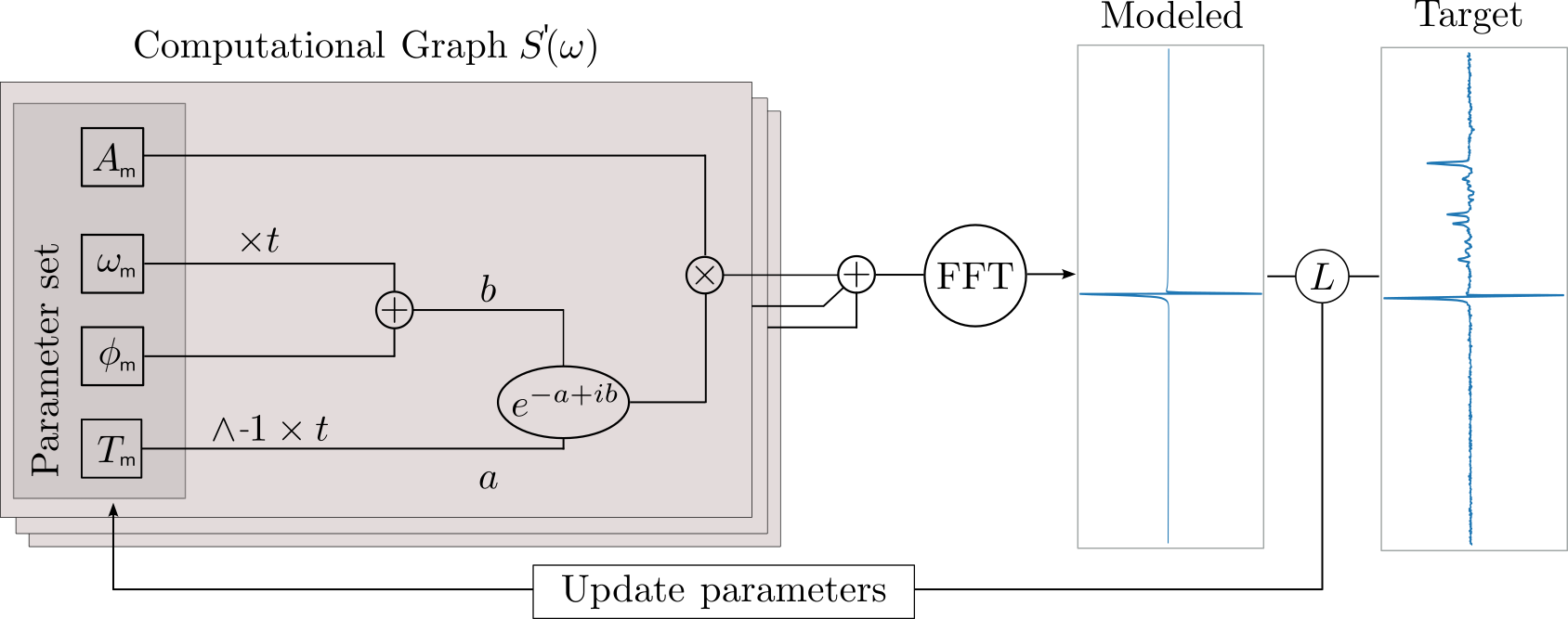
We implemented the fitting pipeline in Python using the Torch library. Our method involves creating a computational graph (i.e., a torch.nn.Module) corresponding to the linear combination of 7 Lorentzian profiles to model the water residuals, given by:

$$$ S'_k(\omega) = FFT( \sum^7_{m=1} A_{m,k}\,e^{(-T^{-1}_{m,k}\,t+2\,i\,\pi(\omega_{m,k}\,t+\phi_{m,k}))}),$$$

where $$$A_{m,k}$$$, $$$\omega_{m,k}$$$, $$$T^{-1}_{m,k}$$$, and $$$\phi_{m,k}$$$ are trainable tensors corresponding to each Lorentzian area, frequency shift, width, and phase, respectively. the spectrum index is represented by k. Each Lorentzian frequency shift was limited between 4.5 and 4.9 ppm, using “torch.clamp”. The error between a simulated spectrum $$$S'_k$$$ and the original spectra $$$S_k$$$ is given by:

$$$ l(S_k(\omega),S'_k(\omega)) = MSE(S_k(\omega_{[4.4,7.0]}), S'_k(\omega_{[4.4,7.0]})) + \sum^7_{m=1} A_{m,k} + ||S'_k(\omega_{[0,4.4]})||^2,$$$

where MSE corresponds to the mean squared error, [4.4, 7.0] corresponds to the considered range in ppm, and k is the spectrum index. The second term corresponds to regularization by each Lorentzian amplitude that helps obtain a smoother residual, while the last term is added to avoid the method substracting a substantial component in the range of interest. Finally, the total Loss is given by:

$$$L = \frac{1}{N} \sum^N_{k=1} l(S_k(\omega), S'_k(\omega)).$$$

The iterative process continues until the error between a set of the simulated spectra $$$S'_k(\omega)$$$ and the N input spectra $$$S(\omega)$$$ is minimized. Finally, we subtract the simulated water residuals from the original spectra. The hyperparameters used for the minimization are: early stopping after ten epochs and a learning rate of 0.01 with Rprop⁴ as the optimizer. Figure 1 shows a representation of the used computational graph, and the implementation will be available at https://github.com/TuchoTurco/Water-Removal.
For evaluating the performance, we used an in-vivo dataset consisting of 3360 spectra acquired with a semiLASER 2D-MRSI pulse for TE 135 and 40 ms at a 3T Siemens scanner. Extra data has been used to test the time performance, consisting of 10000 spectra. The water residual removal was performed with our approach together with HLSVD-PRO. On the results, metabolite quantification was performed on eight metabolites (Cho, Glu, Lac, Gln, Cr, Asp, NAA, and mI), including baseline fitting using p-splines. All the presented results for our method were obtained using a GPU Nvidia GTX 1060, 6Gb with CUDA 11.7 and Torch 1.13.1. HLSVD-PRO was parallelized on 16 cores using an AMD Ryzen 7 2700X processor.

Results

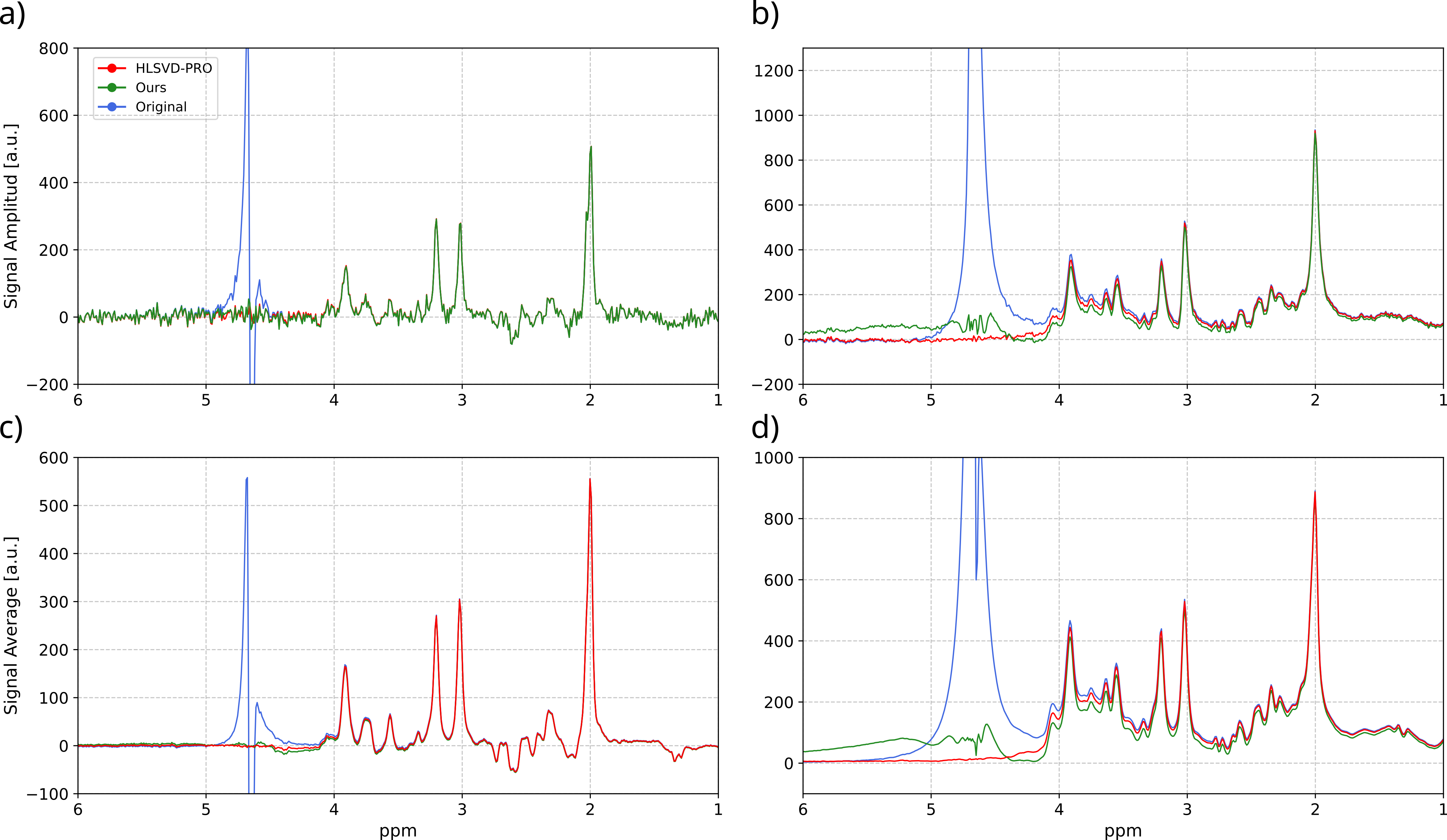
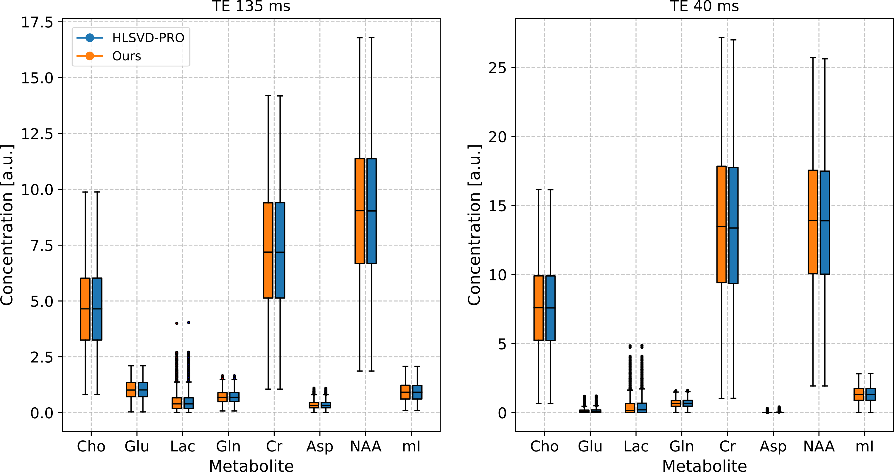
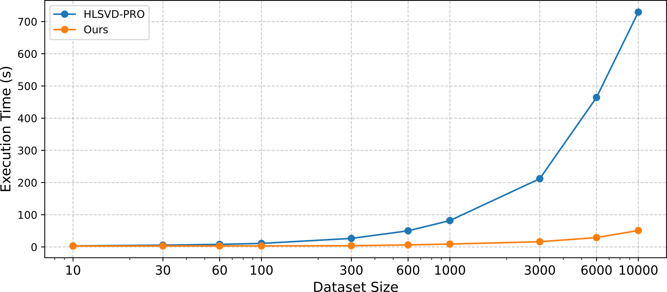
In Figure 2a, we present the output of our method for an echo time (TE) of 135 ms, compared with the HLSVD-PRO and the original spectrum. Figure 2b corresponds to a TE of 40 ms. We found that for long TE, our methods perform similarly to HLSVD, while on shorter TE, the method maintains a substantial residual. This is better represented in Figures 2c and 2d, where the average between all the spectra is shown, where long TE performance is closer to that of HLSVD. Figure 3 shows no significant difference between the spectrum processed with HLSVD and our method for both echo times.
Figure 4 illustrates the time taken by our method running on the GPU and HLSVD parallelized on the CPU as a function of the dataset size. We obtained a speed-up factor of 14x to remove water from 10000 spectra in less than one minute (specifically, 51 seconds), compared with little more than 12 minutes with HLSVD.

Discussion

The use of Torch for parallelized fitting of water residuals in MRSI offers a promising alternative for water removal. Even though the method lacks robustness when applied on short TE, the metabolite quantification obtains similar results due to the use of a baseline. The use of other regularizers must be further analyzed in order to solve this limitation.

Conclusion

The proposed method for accelerating water residual removal in MRSI data by parallelized fitting with Torch presents a viable solution to the time-consuming process of water removal. Its superior time efficiency suggests its potential relevance to clinical practice.

Acknowledgements

The project leading to this application has received funding from the European Union’s Horizon 2020 research and innovation programme under the MarieSklodowska-Curie grant agreement No 813120