2987

On the impact of eddy-current-induced biases in ΔB0 maps on shimming outcomes

Busra Bulut¹, Ismail Foudali², Alexandre D’Astous³, and Eva Alonso-Ortiz³
¹Ecole Nationale Supérieure de Techniques Avancées, Paris, France, ²Georg Simon Ohm University of Applied Sciences, Nuremberg, Germany, ³Polytechnique Montreal, Montreal, QC, Canada

Synopsis

Keywords: Data Processing, Shims

Motivation: Eddy-currents can bias magnetic field (∆B0) maps.

Goal(s): To assess the impact of eddy-current-biased ∆B0 maps on B0 shimming and T2* measurements.

Approach: Measure the shimmed ∆B0 field after having used a ∆B0 map that is thought to be affected by eddy currents vs. one that is obtained using the gradient-reversal technique for canceling eddy-currents. Measure T2* values after using both shimming conditions.

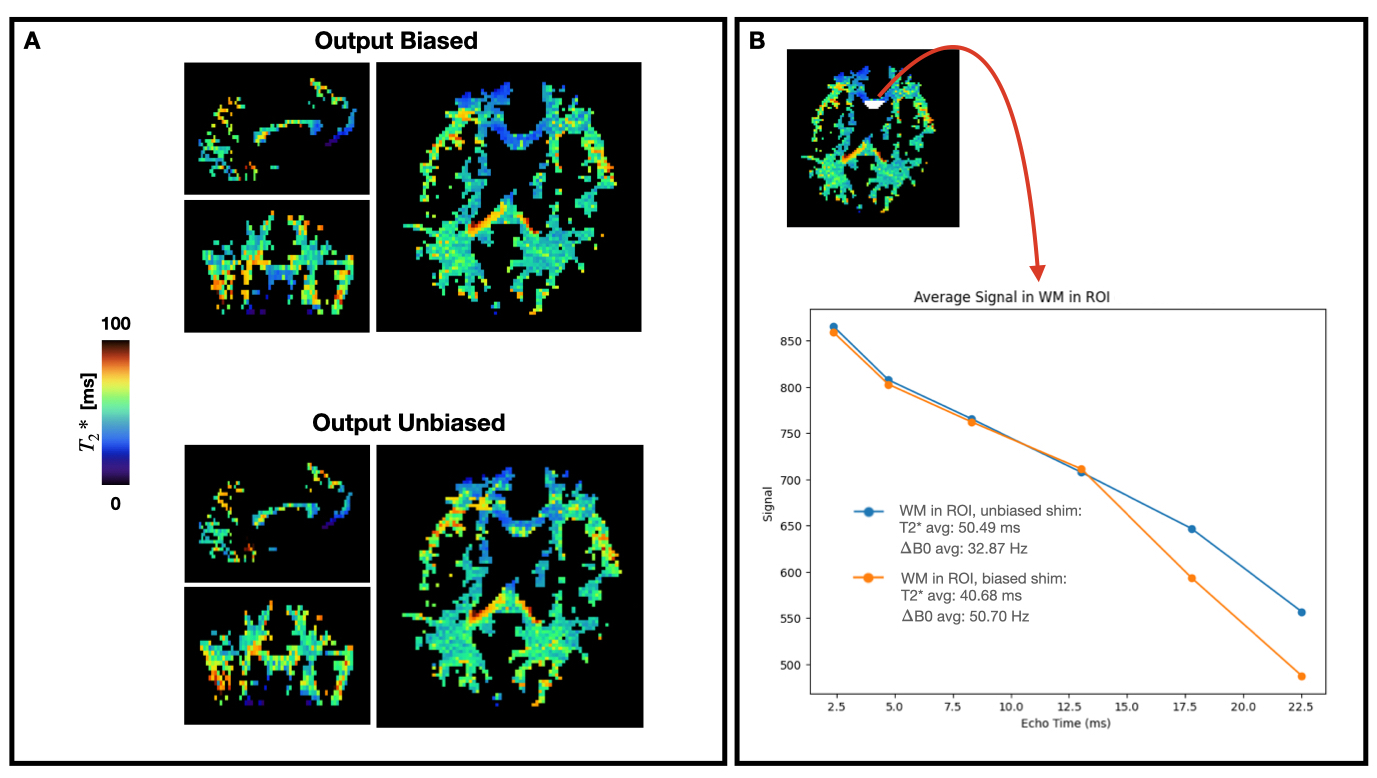
Results: Eddy-currents arising from spatial-encoding gradients have a measurable impact on shim quality and can reduce T2* values in the brain by up to 10 ms.

Impact: Scientists and clinicians interested in measuring T2* in areas that are affected by strong magnetic field inhomogeneities may want to consider that eddy-current-induced biases in ∆B0 maps could lead to reduced T2* in those regions.

Introduction

Magnetic susceptibility (χ) differences in MRI cause non-uniformities in the magnetic field (∆B0) which lead to signal loss. To address this, scanners shim the magnetic field before imaging. This involves measuring ∆B0 (typically using a dual-echo gradient-echo (GRE) sequence) and generating compensatory magnetic fields. Previous 7T work¹ suggests that eddy-currents arising from spatial-encoding gradients cause biases in ∆B0 maps. Here, we sought to identify the degree to which spatial-encoding gradients cause biases in ∆B0 maps at 3T and to assess the impact of biased ∆B0 maps on shimming outcomes.

Methods

Custom Phantom Design: To validate the accuracy of in-vivo ∆B0 mapping protocols, we created a phantom with ∆B0 similar to those reported in the brain (maximum of ~1.6ppm² near air-tissue boundaries). We inserted a plastic cylinder (r=5.9mm, thickness=0.28mm) within an acrylic sphere (r=10cm), filled both compartments with an agar-based gel³, and doped the inner compartment with 27.6mmol/L of Gadovist 1.0 (χ=326 ppm/M^4–9), resulting in a 1.6ppm offset 4mm from the cylinder edge.

Phantom imaging:
Step0: Place a uniform spherical phantom within a 3T Siemens MRI and run the scanner’s default shimming procedure.
Step1:
(a) Replace the uniform phantom with our custom phantom and set the shim settings to those of Step0.
(b) Acquire two multi-slice dual-echo GRE sequences (TR=8.2ms,TE1=3.38ms,TE2=5.58ms,BW=745Hz/pixel,FA=25°,resolution=2x2mm²,2mm slices) with opposing PE, FE, and SS gradient polarities.
Step2:
(a) Create two ∆B0 maps and average them to obtain an eddy-current-free ∆B0 measurement.
(b) The result of Step2a is equal to “output biased” (i.e., ∆B0 after shimming based on a single-polarity ∆B0 map).
(c) Input the averaged ∆B0 map into the Shimming-Toolbox¹⁰ to compute optimal shim coefficients.
Step3: Using the Shimming-Toolbox coefficients, repeat Steps1b-2a to obtain an “output unbiased” ∆B0 map.
Step4: Repeat Steps1-3 with TR=2000ms.

In vivo imaging: Two volunteers were scanned on the aforementioned 3 T MRI.
Step0: Acquire a T1-weighted (T1w) anatomical scan.
Step1:
(a) Run the scanner’s default shimming procedure.
(b) Acquire a multi-slice multi-echo GRE (MGRE) scan (TE=2.34ms,4.72ms,8.28ms, 13.03ms,17.78ms,22.53ms,TR=981ms,BW=735Hz/pixel,FA=25°,resolution=2x2mm2, 3mm slices) for T2* mapping.
(c) Run two 3D dual-echo GRE scans (TE1=2.5ms, TE2=4.5ms, TR=6.9ms, BW=735Hz/pixel,FA=25°,resolution=4x4x4mm3) with opposing PE, FE, and SS gradient polarities. These parameters were set to match the protocol used by the scanner's default shimming procedure.
Step2:
(a) Create two ∆B0 maps from the dual-echo GRE data and average them.
(b) The result of Step2a is equal to “output biased”.
(c) Input the averaged ∆B0 map into the Shimming-Toolbox to compute optimal shim coefficients.
Step3: Using the Shimming-Toolbox coefficients, repeat Steps1b-2a to obtain an “output unbiased” ∆B0 map.

Post-processing: The in-vivo datasets were co-registered using FSL FLIRT¹¹, T2* maps were generated from MGRE scans using qMRLab¹², and white matter (WM) and gray matter (GM) were segmented on the T1w scan using FSL FAST¹³.

Results

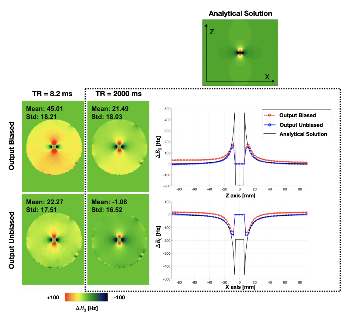
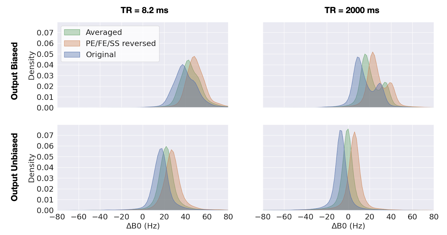
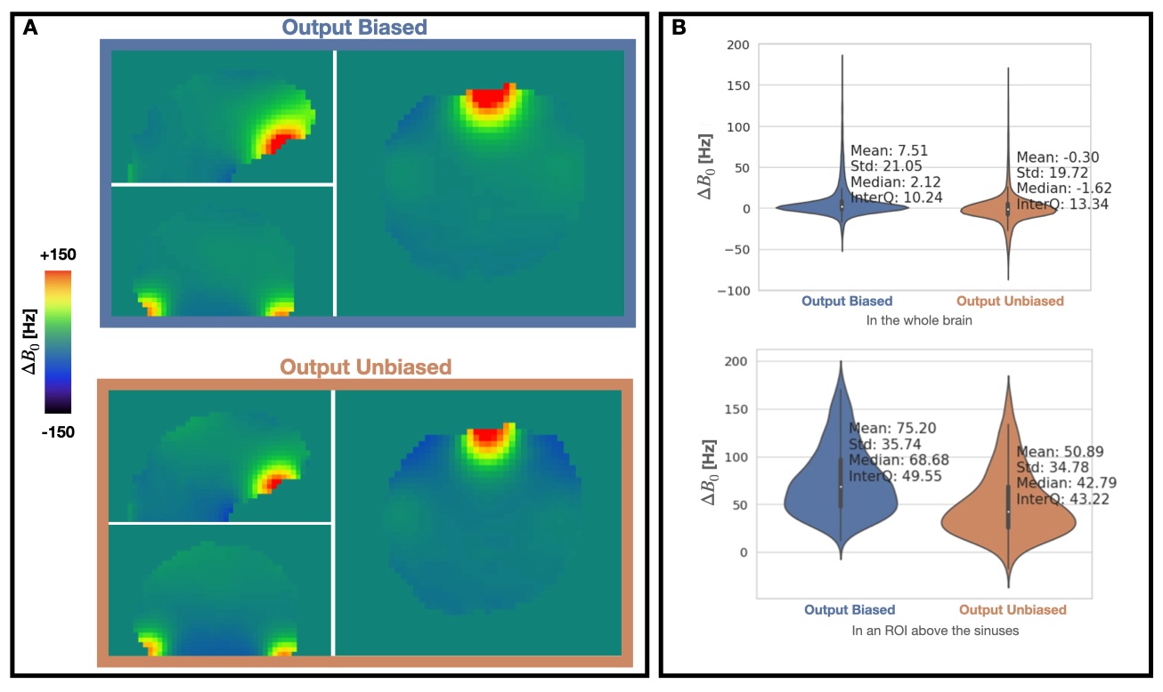
Phantom imaging: In Figures 1-2 we see that when shimming coefficients are computed using a “biased” field measurement, the shimmed ΔB0 field (“output biased”) will have a higher mean and standard deviation (SD) compared to when shimming coefficients are computed using an eddy-current-free (“unbiased”) field map. In the case of the latter and when the TR is long, the shimmed field closely matches the analytical solution for the field.

In-vivo imaging: Results were consistent with phantom findings, in that the ΔB0 field after shimming with an eddy-current bias-free input ΔB0 had a lower overall mean and SD. This effect was more pronounced in brain tissues above the sinuses (Figure 3).
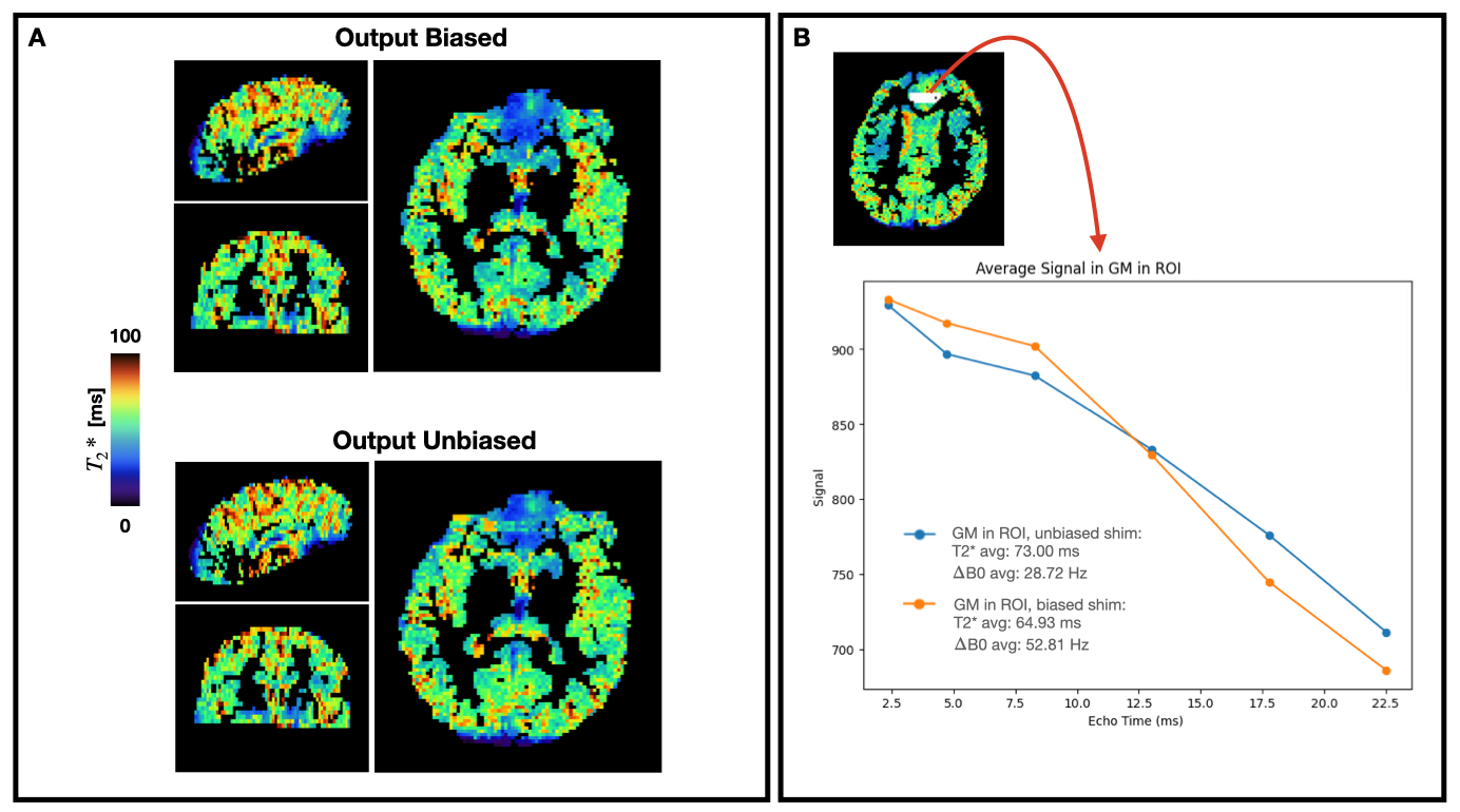
In GM, (Figure 4) we found that when shimming was based on an unbiased ΔB0 map, measured T2* values were 8.07ms higher in an ROI above the sinuses. Similarly, in WM (Figure 5) shimming based on an unbiased ΔB0 map resulted in T2* values that were 9.81ms higher in an ROI above the sinuses.

Discussion and Conclusions

While our long-TR phantom experiments suggest that eddy-current-induced biases in ∆B0 maps can be eliminated by using the gradient-reversal technique, the gradient-reversal technique did not appear to fully eliminate all sources of error in short-TR acquisitions. There may be additional sources of error that decay at long-TR, but do not arise from the encoding gradients. In-vivo, the gradient-reversal technique can improve the quality of the shimmed field. These improvements translate into a T2* recovery of up to 8-10ms in certain frontal brain regions. We performed additional experiments on a uniform phantom comparing ∆B0 with alternate PE/FE-gradient polarities and found no measurable impact (data not shown). Consequently, we attribute the biases in the presented ∆B0 maps to arise primarily from eddy-currents associated with SS-gradients.

Acknowledgements

This work is supported by the TransMedTech Institute, thanks to the financial support of the Canada First Research Excellence Fund and the Fonds de recherche du Québec, the Natural Sciences and Engineering Research Council of Canada (NSERC), and Polytechnique Montreal.

References

1. Varadarajan, D. et al. Characterizing the acquisition protocol dependencies of B0 field mapping and the effects of eddy currents and spoiling. in Proc. Int. Soc. Magn. Reson. Med vol. 29 3552 (2021).

2. Gach, H. M., Curcuru, A. N., Mutic, S. & Kim, T. B0 field homogeneity recommendations, specifications, and measurement units for MRI in radiation therapy. Med. Phys. 47, 4101–4114 (2020).

3. Duan, Q. et al. Characterization of a dielectric phantom for high-field magnetic resonance imaging applications. Med. Phys. 41, 102303 (2014).

4. Fruytier, A.-C. et al. Dynamic contrast-enhanced MRI in mice at high field: estimation of the arterial input function can be achieved by phase imaging. Magn. Reson. Med. 71, 544–550 (2014).

5. Olsson, E., Wirestam, R. & Lind, E. MRI-Based Quantification of Magnetic Susceptibility in Gel Phantoms: Assessment of Measurement and Calculation Accuracy. Radiol. Res. Pract. 2018, 6709525 (2018).

6. Hwang, S. & Lee, S. K. Efficient experimental design for measuring magnetic susceptibility of arbitrarily shaped materials by MRI. Investigative Magnetic Resonance (2018).

7. de Rochefort, L., Brown, R., Prince, M. R. & Wang, Y. Quantitative MR susceptibility mapping using piece-wise constant regularized inversion of the magnetic field. Magn. Reson. Med. 60, 1003–1009 (2008).

8. Deh, K. et al. Multicenter reproducibility of quantitative susceptibility mapping in a gadolinium phantom using MEDI+0 automatic zero referencing. Magn. Reson. Med. 81, 1229–1236 (2019).

9. Hsieh, C.-Y., Cheng, Y.-C. N., Neelavalli, J., Haacke, E. M. & Stafford, R. J. An improved method for susceptibility and radius quantification of cylindrical objects from MRI. Magn. Reson. Imaging 33, 420–436 (2015).

10. D’Astous, A. et al. Shimming-Toolbox: An open-source software package for performing realtime B0 shimming experiments. Magn. Reson. Med. 89(4), 1401-1417(2023).

11. Jenkinson, M. & Smith, S. A global optimisation method for robust affine registration of brain images. Med. Image Anal. 5, 143–156 (2001).

12. Karakuzu, A. et al. qMRLab: Quantitative MRI analysis, under one umbrella. Journal of Open Source Software 5, 4 (2020).

13. Zhang, Y., Brady, M. & Smith, S. Segmentation of brain MR images through a hidden Markov random field model and the expectation-maximization algorithm. IEEE Trans. Med. Imaging 20, 45–57 (2001).

Figures

The 4 images on the left show ΔB0 after shimming based on a single-polarity ΔB0 map (top row, “output biased”) and an opposing-polarity-averaged ΔB0 map (bottom row, “output unbiased”). The ΔB0 maps in the left column were shimmed using short-TR ΔB0 maps and those in the right column were shimmed using long-TR ΔB0 maps. To the right, we have the ΔB0 profile along a central line of the z-axis (head-foot) and x-axis (left-right) when shimming with long-TR biased (red) and unbiased (blue) ΔB0 maps. The solid line indicates the analytically-predicted ΔB0 (also shown on the topmost figure).

Kernel Density Estimate (KDE) plots used to show ΔB0 distributions across the same slice in maps that were shimmed using short and long-TR measurements that are either based on a single encoding-gradient polarity (“output biased”) or based on averaged opposing-polarities (“output unbiased”). To avoid biases in the measurement of the shimmed field, the average (green distributions) of opposing-polarities (“PE/FE/SS reversed”: red distributions and “Original”: blue distributions) approach is also used to measure the shimmed field.

(A) ΔB0 maps after shimming based on a single encoding-gradient polarity (“output biased”) vs. based on averaged opposing-polarities (“output unbiased”). (B) Distribution of ΔB0 values in output biased (blue distributions) and unbiased (orange distributions) maps across the whole brain (top) and an ROI above the sinuses (bottom).

(A) T2* maps in GM after shimming based on a single encoding-gradient polarity (“output biased”) vs. based on averaged opposing-polarities (“output unbiased”). (B) Average MGRE signals across echo times in a GM ROI for a biased (orange) vs. unbiased (blue) shim. The measured T2* time for each shim condition is reported alongside the average ΔB0 offset in the ROI.

(A) T2* maps in WM after shimming based on a single encoding-gradient polarity (“output biased”) vs. based on averaged opposing-polarities (“output unbiased”). (B) Average MGRE signals across echo times in a WM ROI for a biased (orange) vs. unbiased (blue) shim. The measured T2* time for each shim condition is reported alongside the average ΔB0 offset in the ROI.

Proc. Intl. Soc. Mag. Reson. Med. 32 (2024)

2987

DOI: https://doi.org/10.58530/2024/2987