2954
Microstructure-informed brain segmentation in multiple sclerosis using CAQE1University of British Columbia, Vancouver, BC, Canada, 2MR Clinical Science, Philips Healthcare Canada, Missisauga, ON, Canada, 3International Collaboration on Repair Discoveries, Vancouver, BC, Canada
Synopsis
Keywords: Multiple Sclerosis, Microstructure
Motivation: Progression in neurodegenerative diseases such as multiple sclerosis (MS) involves tissue damage invisible on conventional MRI scans. Quantitative measures of tissue microstructure may be more informative.
Goal(s): To segment MS brain MRI data based on quantitative microstructural MRI measures without spatial input.
Approach: 23 MS brain scans were segmented based on clustering healthy quantitative data using an unsupervised Clustering for Anatomical Quantification and Evaluation (CAQE) framework. Classifications of lesions and normal appearing tissue were compared to a healthy atlas segmentation.
Results: MS brains showed several differences from healthy classification in normal-appearing regions on conventional MRIs. Periventricular lesions were generally classified consistently.
Impact: Using only microstructural features, the CAQE framework can classify diseased tissue in more detail than conventional segmentation algorithms based on qualitative MRI scans, and provide useful information for improved diagnosis, follow-up and more personalized care.
Introduction
Multiple sclerosis (MS) is an autoimmune inflammatory and demyelinating disease characterized by focal lesions; however lesion burden is only weakly correlated with clinical disease progression1. Quantitative MRI metrics such as myelin water fraction (MWF)2, and tensor-valued diffusion encoding (TVDE)-derived microscopic fractional anisotropy (µFA)3 and CMD3, a measure of tissue heterogeneity, may help provide useful information regarding brain microstructure. Here we use an unsupervised segmentation approach, Clustering for Anatomical Quantification and Evaluation (CAQE), to segment MS brains, based only on microstructural features without spatial input.Methods
Acquisition25 healthy participants (mean=46y, 11M/14F), 10 relapsing-remitting MS (RRMS, mean=50y, 3M/7F), 4 secondary progressive MS (SPMS, mean=65y, 4F) and 9 primary progressive MS (PPMS, mean=62y, 4M/5F) at 3T underwent:
- T1w: 3D TFE (1x1x1mm3, ~3.5 minutes)
- FLAIR: 3D TIR (1x1x1mm3, ~5.5 minutes) for MS only
- MWF Imaging: CALIPR4 (56 echoes, acquired at 1.7x1.7x1.7mm3, ~7.5 minutes)
- TVDE: Spherical (33 directions, ~3 minutes), planar (32 directions, ~3 minutes) and linear tensor encoding (59 directions, ~5 minutes) at 3x3x3mm3, bmax=2000s/mm2.
Processing
MWF maps were generated using a 3D spatial correlation-based analysis5. Maps of µFA and CMD were generated using the QTI+ framework6. Atlases of MWF, µFA and CMD were generated from all healthy participant data7 to provide a population average for comparison with MS. For all participants, CSF was masked out and metric maps were registered to each individual’s MWF space.
Segmentation
25 healthy participants’ quantitative MRI data were randomly divided into a training (n=20) and testing (n=5) set, and training data was clustered using a Fuzzy C-Means algorithm8 to label datapoints. Each test dataset was then classified based on clustering using a K-Nearest Neighbours (KNN) algorithm9. The healthy metric atlases were classified based on clustering all healthy participants, to provide a population-averaged comparison for MS. The “best” number of clusters for healthy data was determined using Davies-Bouldin and Calinski-Harabasz scores. Based on clustering healthy data, MS data was classified with a KNN algorithm. The optimal number of clusters was not expected to be the same for MS and healthy data, so higher cluster numbers were also attempted.
Results
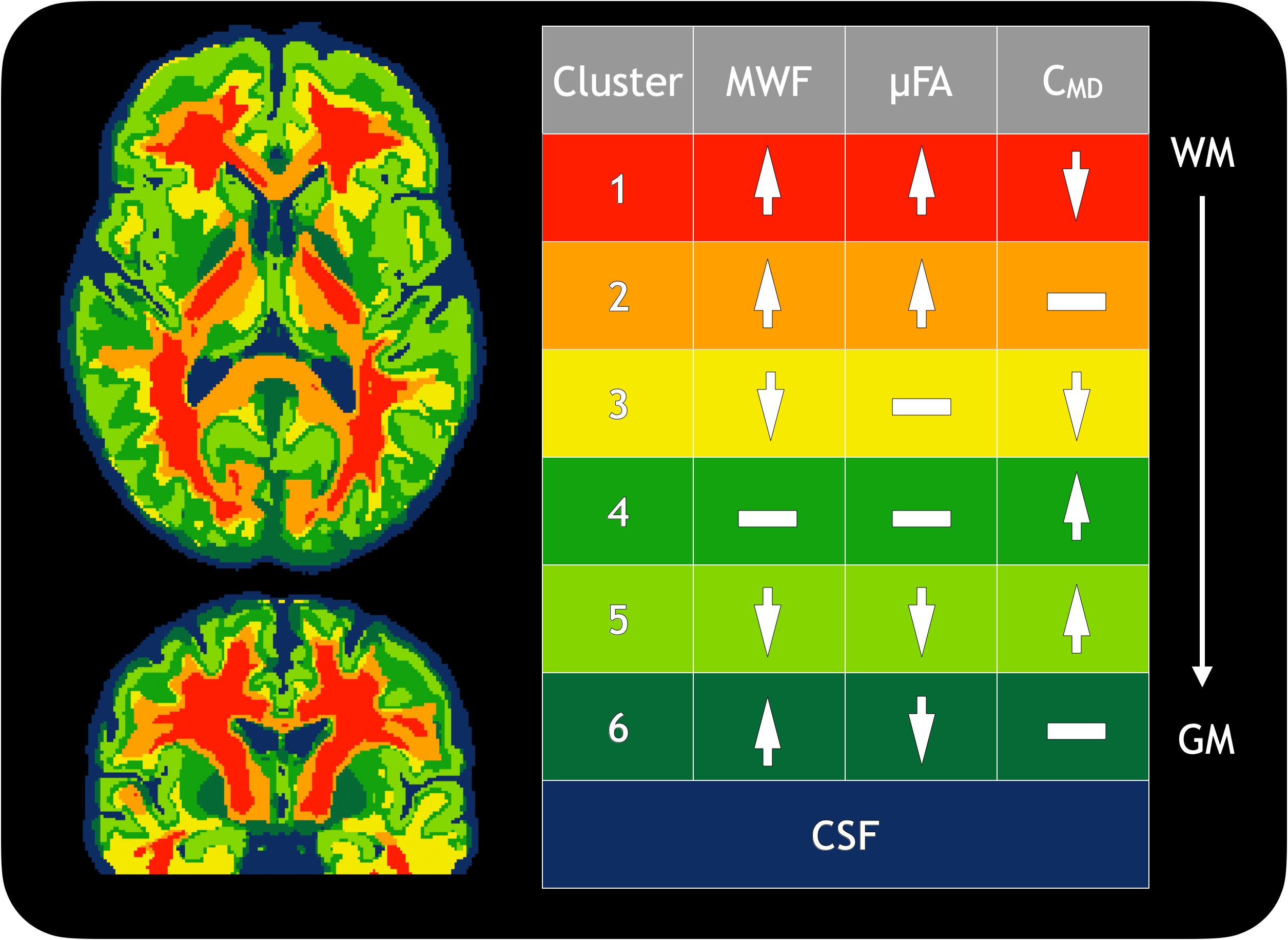
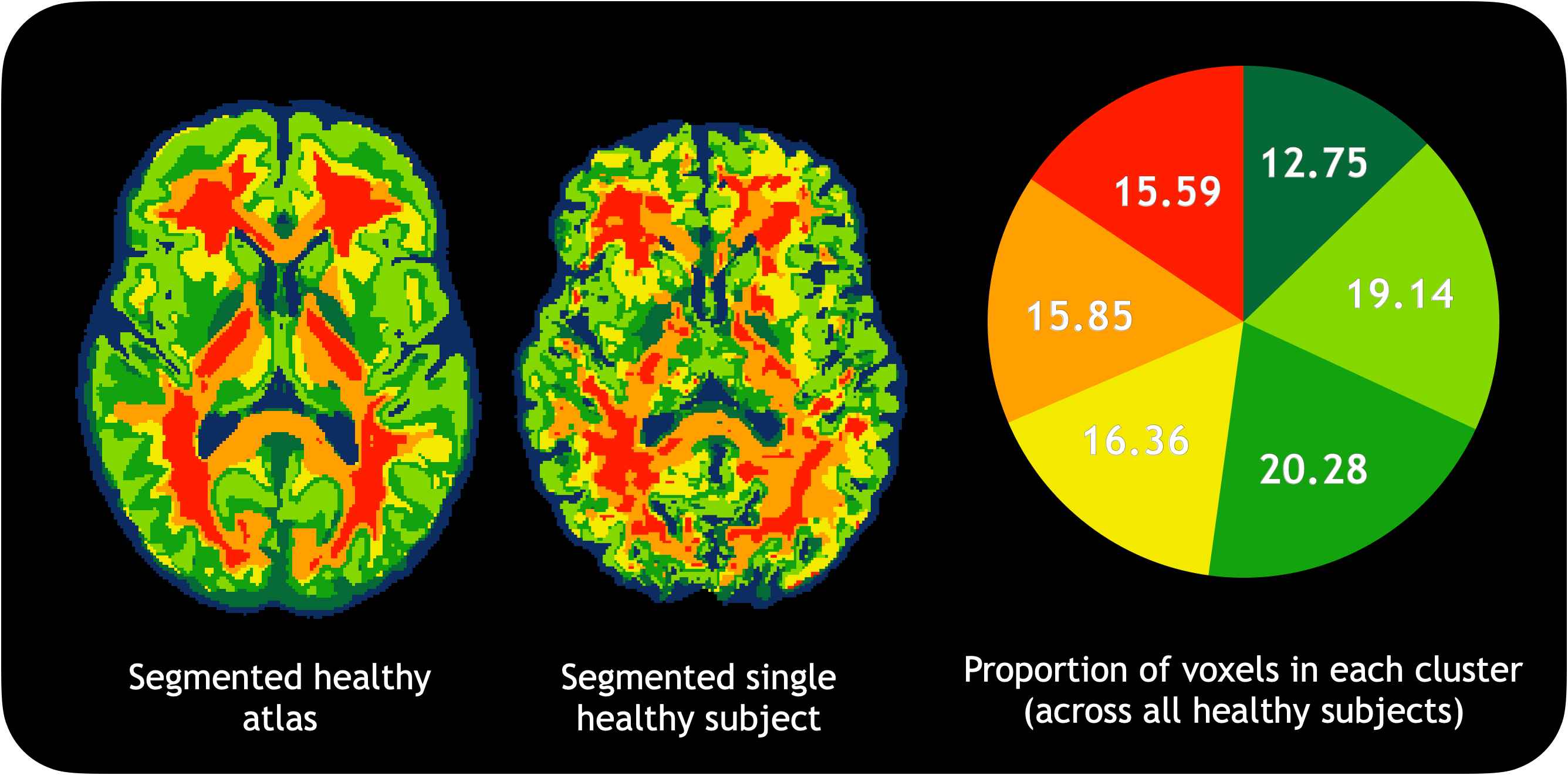
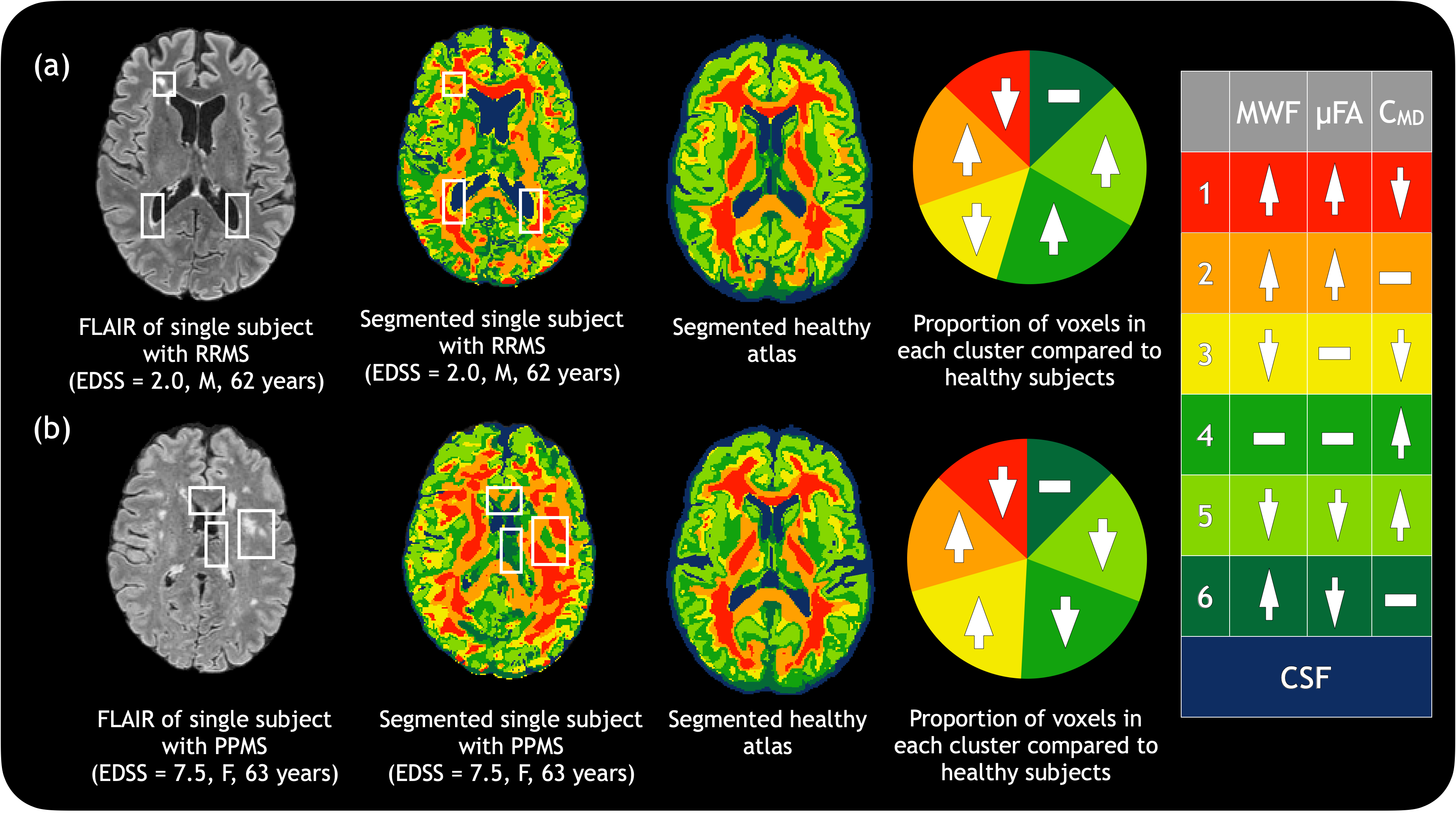
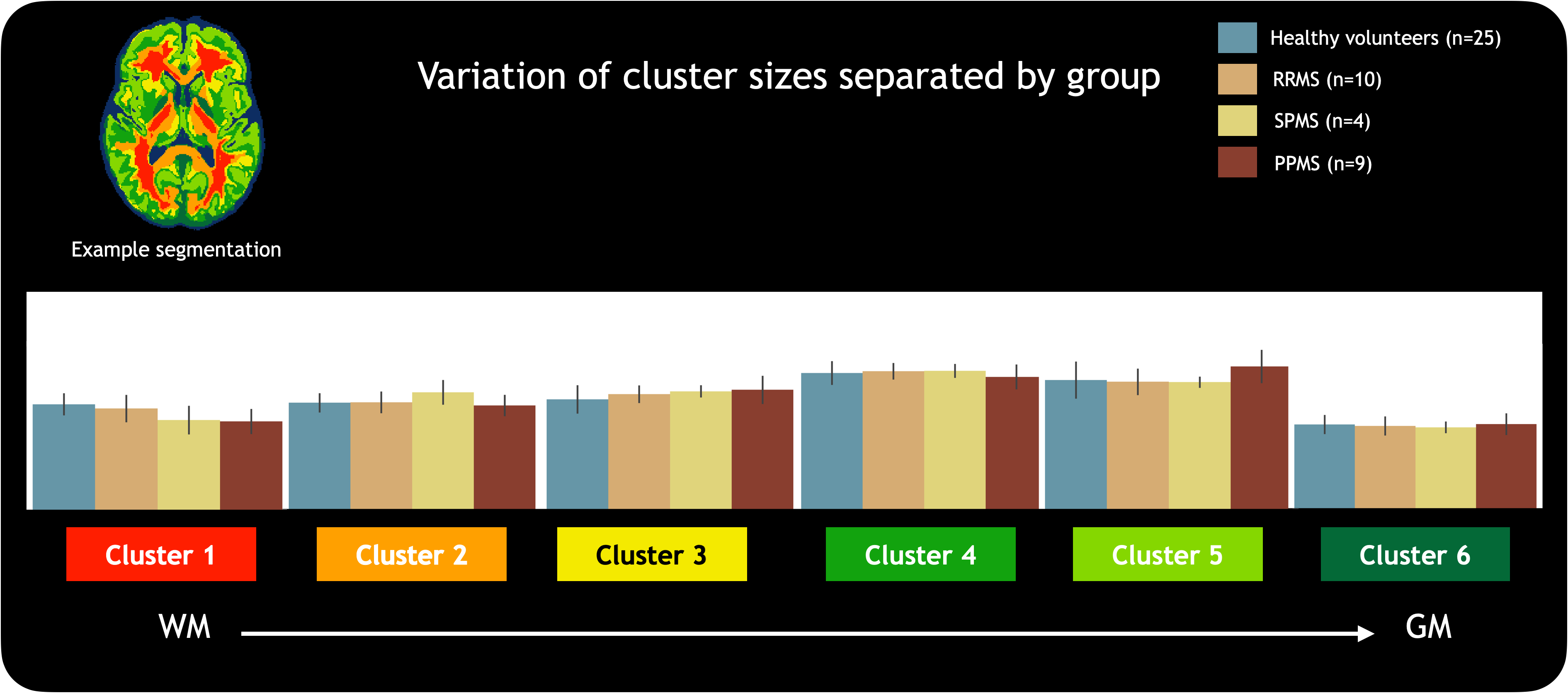
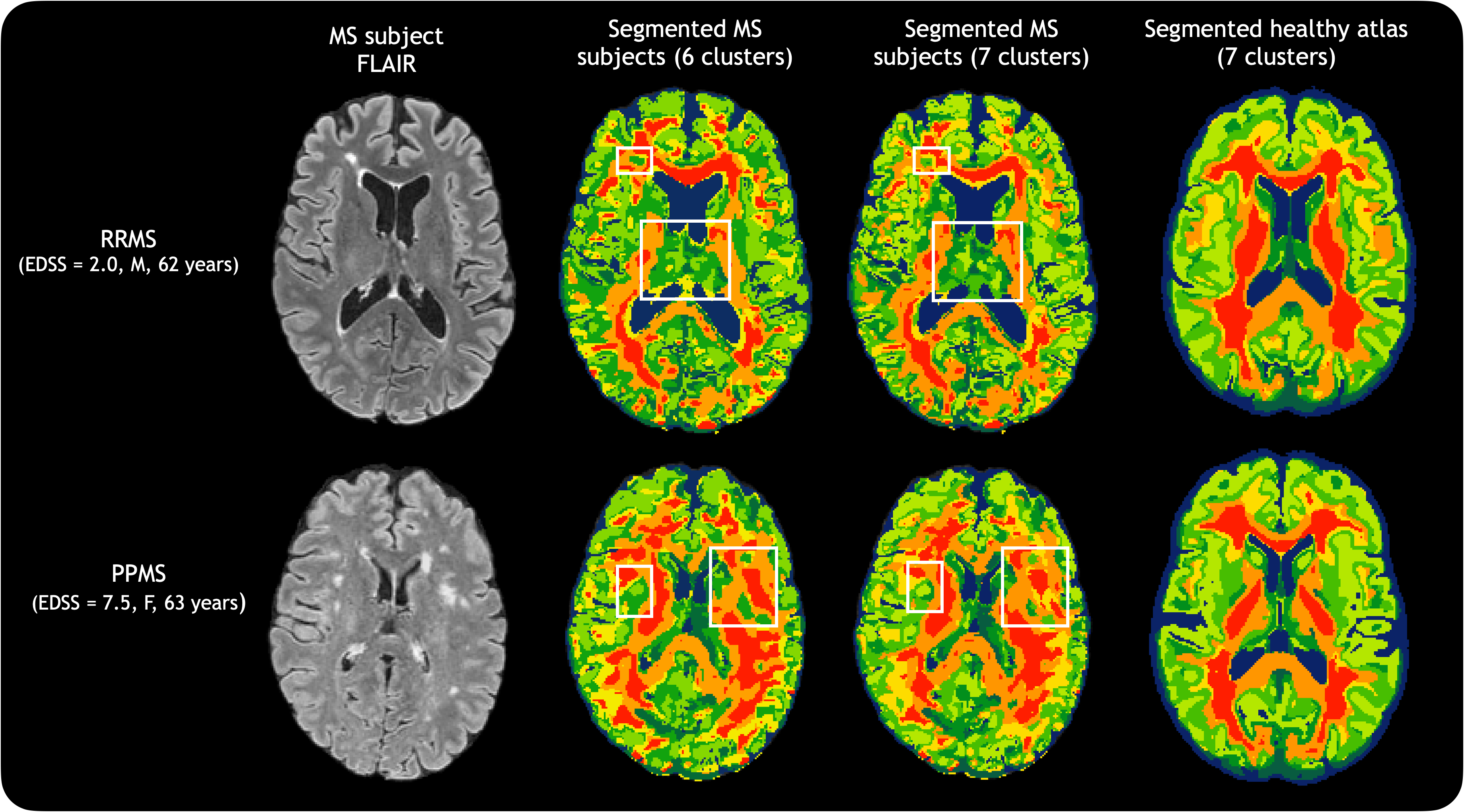
Figure 1 presents the segmented atlas and a table of relative mean metric values; 6 clusters were preferred across healthy participants. Figure 2 shows the segmented atlas alongside a single segmented healthy brain, with proportions of cluster sizes across all healthy people. Figure 3 demonstrates two examples of MS clustering. Figure 4 shows how cluster sizes varied by group. Figure 5 highlights how segmentations would change in MS if 7 clusters were used instead of 6. Clustering was driven by µFA (explained variance ratio 46%) followed by CMD (34%) and MWF (20%). One-way ANOVA showed a difference between groups in Cluster 1.Discussion
The metrics chosen for the CAQE approach (MWF, µFA, CMD) were known to include largely complementary information10, providing a broad spread of information for clustering. In healthy participants, consistent patterns of clusters were observed. Cluster proportions varied slightly between the different groups, with #1 showing a significant difference between SPMS/PPMS and healthy data.In MS, the overall patterns remained consistent, but in areas of damage or disruption, regions were marked as more grey matter-like; e.g., in Figure 3a, the top left lesion was marked as having moderate MWF and µFA, and high CMD. Periventricular lesions largely presented as #3 (yellow, representing low MWF, moderate µFA and low CMD), perhaps indicating demyelination and the beginnings of axonal damage (indicated by decreased µFA). Subjects with higher EDSS scores (e.g. Figure 3b) sometimes showed deep grey matter regions as #6, which likely represents artificially high MWF due to high iron concentration. In Figure 5, using 7 rather than 6 clusters, some types of tissue damage were further separated.
Applying the CAQE framework to disease is limited by training on healthy data; possible directions include training on MS data, or using more clusters. Clusters must be interpreted with caution, as they include different microstructural features. In our data, the low resolution of TVDE may have missed some lesions. Despite these drawbacks, CAQE shows promise as a tool to compare MS tissue classification against a healthy average.
Conclusion
The CAQE framework can be used to segment MS brains based on quantitative MRI-derived microstructural measures. MS classifications highlighted lesions and areas of other tissue damage. Future work could include using different metrics with CAQE and more clusters to better characterize MS tissue abnormalities.Acknowledgements
We thank study participants and the UBC MRI Research Centre’s MR technologists and staff for their time and support. SB is funded by a Natural Sciences and Engineering Research Council (NSERC) Canada Graduate Scholarship- Doctoral; SHK is funded by Canadian Institute for Health Research (CIHR), Multiple Sclerosis Canada, NSERC. GG is an employee of Philips Canada.References
1. Chard D, Trip SA. Resolving the clinico-radiological paradox in multiple sclerosis. F1000Res. 2017 Oct 12;6:1828. doi: 10.12688/f1000research.11932.1.
2. Mackay, A., Whittall, K., Adler, J., Li, D., Paty, D. and Graeb, D. (1994), In vivo visualization of myelin water in brain by magnetic resonance. Magn. Reson. Med., 31: 673-677. https://doi.org/10.1002/mrm.1910310614
3. Westin CF, Knutsson H, Pasternak O, Szczepankiewicz F, Özarslan E, van Westen D, Mattisson C, Bogren M, O'Donnell LJ, Kubicki M, Topgaard D, Nilsson M. Q-space trajectory imaging for multidimensional diffusion MRI of the human brain. Neuroimage. 2016 Jul 15;135:345-62. doi: 10.1016/j.neuroimage.2016.02.039.
4. Dvorak AV, Kumar D, Zhang J, Gilbert G, Balaji S, Wiley N, Laule C, Moore GRW, MacKay AL, Kolind SH. The CALIPR framework for highly accelerated myelin water imaging with improved precision and sensitivity. Sci. Adv. 9,eadh9853(2023).DOI:10.1126/sciadv.adh9853
5. Kumar D, Hariharan H, Faizy TD, Borchert P, Siemonsen S, Fiehler J, Reddy R, Sedlacik J. Using 3D spatial correlations to improve the noise robustness of multi component analysis of 3D multi echo quantitative T2 relaxometry data. NeuroImage 2018;178:583--601. https://doi.org/10.1016/j.neuroimage.2018.05.026
6. Herberthson M, Boito D, Haije TD, Feragen A, Westin CF, Özarslan E. Q-space trajectory imaging with positivity constraints (QTI+). Neuroimage. 2021 Sep;238:118198. doi: 10.1016/j.neuroimage.2021.118198.
7. Avants BB, Yushkevich P, Pluta J, Minkoff D, Korczykowski M, Detre J, Gee JC. The optimal template effect in hippocampus studies of diseased populations. Neuroimage. 2010 Feb 1;49(3):2457-66. doi: 10.1016/j.neuroimage.2009.09.062.
8. Warner J, Sexauer J, scikit-fuzzy, twmeggs, alexsavio, Unnikrishnan A, Castelão G, Pontes FA, Uelwer T, pd2f, laurazh, Batista F, alexbuy, Van den Broeck W, Song W, The Gitter Badger, Pérez RAM, Power JF, Mishra H, … 99991. (2019). JDWarner/scikit-fuzzy: Scikit-Fuzzy version 0.4.2 (v0.4.2). Zenodo. https://doi.org/10.5281/zenodo.3541386
9. Fabian P, Gaël V, Alexandre G, Vincent M, Bertrand T, Olivier G, Mathieu B, Peter P, Ron Weiss, Vincent D, Jake V, Alexandre P, David C, Matthieu B, Matthieu P, Édouard D; JMLR. 12(85):2825−2830, 2011.
10. Balaji S, Dvorak AV, Wiley N, MacMillan EL, Traboulsee A, Vavasour IM, Gilbert G, Moore GRW, Li DKB, Laule C, MacKay AL, Kolind SH. Painting a more complete picture of brain microstructure with myelin water fraction and microscopic fractional anisotropy. Under review, submitted Sep 27 2023.
Figures