Introduction

Achieving spatial precision in a measurement system without the use of magnetic components is essential to characterize physical parameters inside a magnet bore. Such solutions can be expensive¹, may compromise its versatility and ability to cater to a wide range of applications. Motivated by the COSI measure design¹, we advance the robot features by making it cost-effective (<$2000), scalable to 16 analog channels(sensors) and a standalone system by employing system-on-chip (SoC) architecture.

Methods

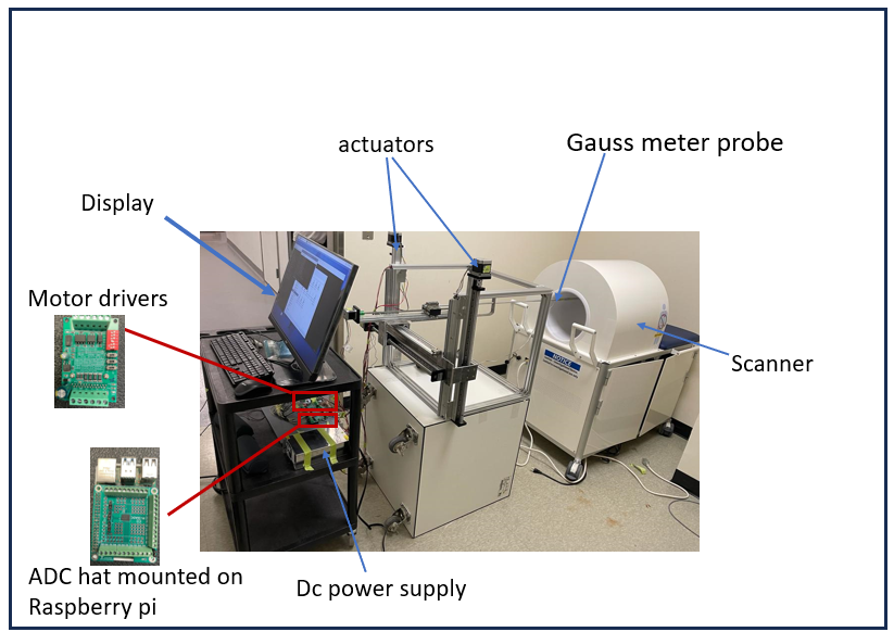
a) Mechanical subsystem: Figure 1 shows the setup.
The mechanical subsystem was designed to deliver a sturdy three-axis linear stage, featuring an aluminum frame crafted from 11 individual aluminum profiles, each with dimensions of 500x40x20 mm³. The system as a whole measures 580 × 540 × 500 mm³. To facilitate linear movement, four linear actuators were integrated, with two exclusively serving the z-axis, one for the y-axis, and the other for the x-axis, producing a 500mm stroke length. These linear actuators were securely affixed to custom-made 10mm thick aluminum plates. Linear guides were employed to steer and support the mechanical motion.
b) Electronic system:
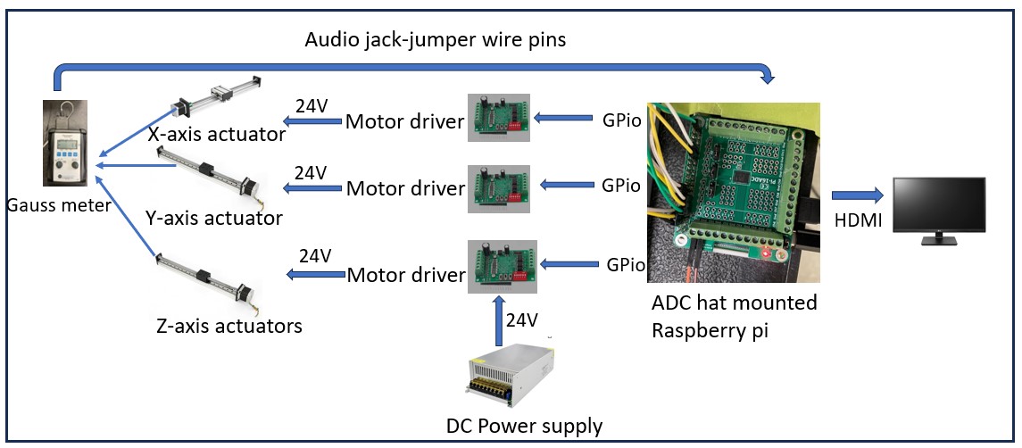
Figure 2 shows the electrical setup of the system.The Raspberry Pi (RPi 4 Model B) served as the central component of the electronic subsystem, providing real-time control over the motor drivers. It was powered by a 5V DC source.. Four motor drivers were used to control the movements of the four linear actuators. These drivers are powered by 24V from a 24V AC/DC power supply unit (Digishuo). The motor drivers supply 24 volts to the linear actuators.
c) Firmware and software:
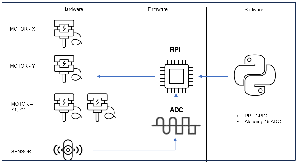
Figure 3 shows the firmware/software components and the libraries used to control the robot. We leveraged the RPi’s general purpose input output (GPIO) library to control the inputs to the stepper motor by setting the direction (clockwise or anti-clockwise) and the number of steps to move. The step-count to traverse 5mm was calibrated using a ruler. The Gauss meter measurement was read in by using a 16 channel ADC hat (Alchemy Power Inc., USA). The rastering of the measurement points was performed using the numpy library. The SoC feature of the RPi enabled the system to be a small footprint, standalone robot and did not require any external computer for control or display. We leveraged the RPi’s inbuilt interfaces for these tasks.
d)Measurements:
The Gauss meter probe was mounted on the robot rod (Figure 1) and was positioned at the midpoint on one edge of the scanner using the software. This was set as the ‘home’ position.. . The measured volume in the three orthogonal axes was 300x170x170 mm³ respectively, with a resolution of 10 mm isotropic. The total measurement time was 4 hours and 49 minutes t. The robot provides a sub-millimeter resolution of 0.02 mm in the x-axis, 0.012 mm in both the y- and z- axes corresponding to one step of the motor in those directions. We also performed a B0 mapping experiment by placing the phantom at 200mm from the bore edge. We used 3D turbo spin echo with acquisition parameters:TR/TE-500/20ms, Matrix-48x48x48, FOV-240x240x240mm3 echo train length (ETL)-4, bandwidth-50kHz. We have acquired two scans with an echo shift of 1 and 50μs to reconstruct the B0 map. The total scan time for both the scans was 12 minutes.

Results

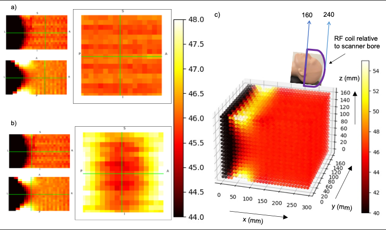
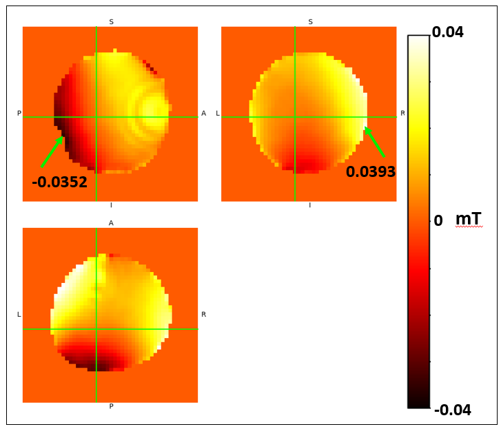
All the materials necessary for the robot’s construction are readily available. This aluminum frame can be easily fabricated and assembled. It provides a working volume of 400x400x350 mm³.The probe holder can support a maximum load of 15 kg. Figure 4 shows the mapped magnetic field of a very low field scanner with a bore length of 530mm; Figure 4a shows the three orthogonal planes centered at a point at iso-center with corresponding images for a point in the fringe field (4b). Figure 4c shows the mapping of the entire volume relative to the placement of the head coil. The magnet appears homogeneous beyond 100mm with a magnetic field of ~46.5mT. Figure 5 shows the B0 map of a spherical phantom that contains water and nickel sulfate with a resolution of 5x5x5mm³ and is similar to the field shown in Figure 4.The green arrows on the maps show the minimum and the maximum B0 offset.

Discussion and future work

We designed, built and demonstrated an automated 3D robot, capable of achieving sub-millimeter-level spatial precision for magnetic field mapping. The robot can potentially integrate other MR compatible sensors for temperature, pH, humidity among others using its 16 channel ADC capability. The authors will deposit the relevant materials including hardware design, component list, and software will be shared on GitHub.

References

1.Han, Haopeng et al. “Open-Source 3D Multipurpose Measurement System with Submillimeter Fidelity and First Application in Magnetic Resonance.” Scientific reports vol. 7,1 13452. 18 Oct. 2017, doi:10.1038/s41598-017-13824-z