Purpose

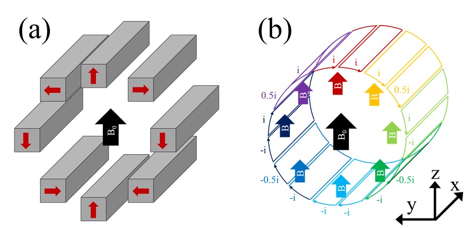
Figure 1a shows a circular Halbach array creating a uniform B₀ field inside a cylinder. The magnetic field direction in loop coils is typically shaped by their geometry. However, by adjusting individual coil currents, we can control this direction, making a cylindrical loop array behave like a Halbach array. Figure 1b visually outlines this process. The loop coil array not only yields a uniform B₀ field but can also generate linear gradients. Cooley et al. introduced a method to achieve uniform fields with directional gradients using Halbach cylinder arrays¹. In contrast, loop coil arrays offer easy control over gradient field direction by adjusting individual coil currents². Our study designed an multi-element loop coil array for uniform B₀ and linear gradients. Current values for uniform field creation were determined via B₀ shimming simulations. We also proposed methods for calculating current strengths to control B₀ field direction and add gradient fields.

Methods

The magnetic field maps of the 8-elements loop coil array were calculated using Biot-Savart’s law. These maps were than organized into matrix A, where each coil's magnetic field contributions to the N voxels were represented as a column vector in A. corresponding current values I_i for each coil were organized in vector I, and the combined magnetic field was calculated as$$\textbf{B}=\textbf{A}\textbf{I}.$$ Uniformity U of B was determined using the equation³$$U=\frac{max(\textbf{B})-min(\textbf{B})}{max(\textbf{B})+min(\textbf{B})},$$and the shim currents were optimized to minimize U, while adhering to current limits $$$(||I_i^{shim}||\leq{I}_{max})$$$ during simulation. The direction of magnetic field could also be controlled by adjusting the shim current. To achieve this, the current values for each coil were adjusted counterclockwise to change the magnetic field direction, which could be accomplished incrementally with a step angle $$$\alpha_s=2\pi/M$$$, where M is the number of coil elements. For the angle between 0 and $$$\alpha_s$$$, required current can be obtained as a liner function relationship. In general, the coil current I can be calculated as$$\left\{\begin{matrix}{I_i=\frac{M(I_{q+1}^{shim}-I_{q+2}^{shim})}{2\pi}\alpha_r+I_{q+2}^{shim}},&{i>1+q,}\\{I_i=\frac{M(I_{q+M+1}^{shim}-I_{q+2}^{shim})}{2\pi}\alpha_r+I_{q+2}^{shim}},&{i=1+q,}\\{I_i=\frac{M(I_{q+M+1}^{shim}-I_{q+M+2}^{shim})}{2\pi}\alpha_r+I_{q+M+2}^{shim}},&{i<1+q,}\end{matrix}\right.$$where q and $$$\alpha_r$$$ are the quotient and remainder of $$$\alpha$$$ divide by $$$\alpha_s$$$, respectively.
Furthermore, the loop coil array can be adapted for 2-axis gradient coils by adjusting the current. To apply G_z gradient, the current is increased from I₁ to I_M/2 and decreased for the rest. The current for each coil can be adjusted using:$$\left\{\begin{matrix}I_i^G=(1+G)I_i,&i\leq\frac{M}{2},\\I_i^G=(1-G)I_i,&i>\frac{M}{2},\end{matrix}\right.$$where G is the gradient weighting factor, and the larger the value, the stronger the gradient. The direction of the gradient field can be changed similarly to using Equation 3.
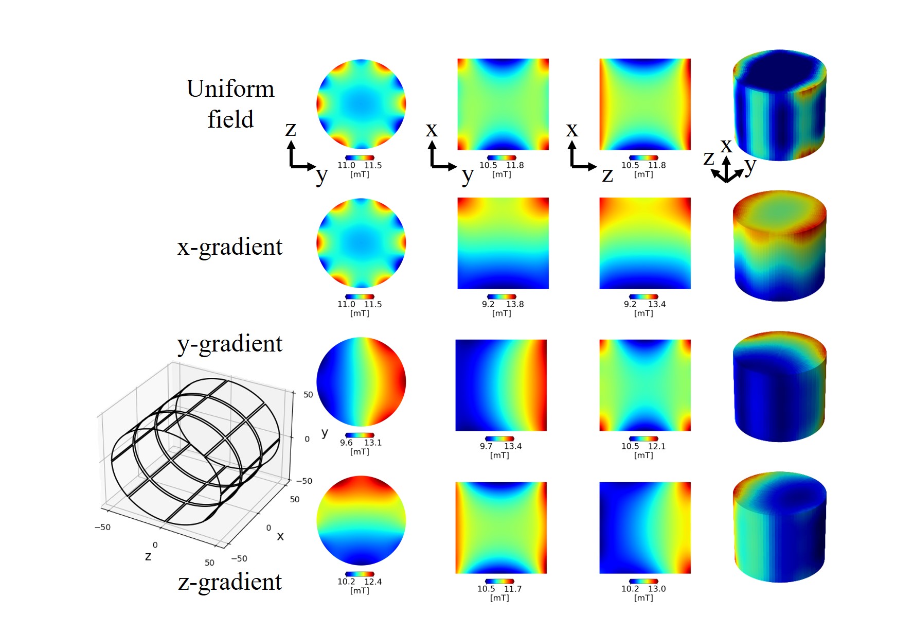
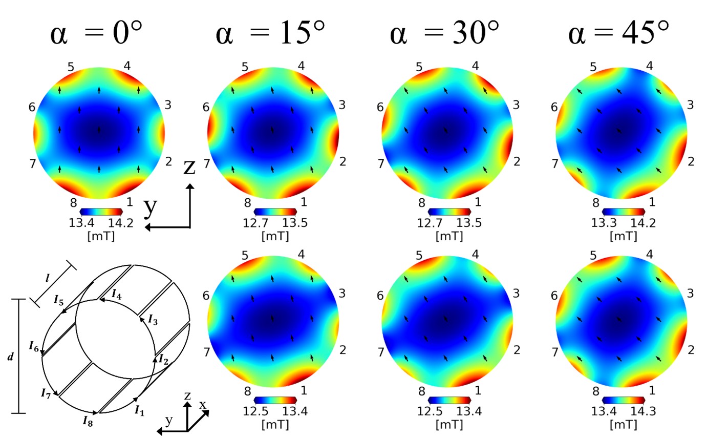
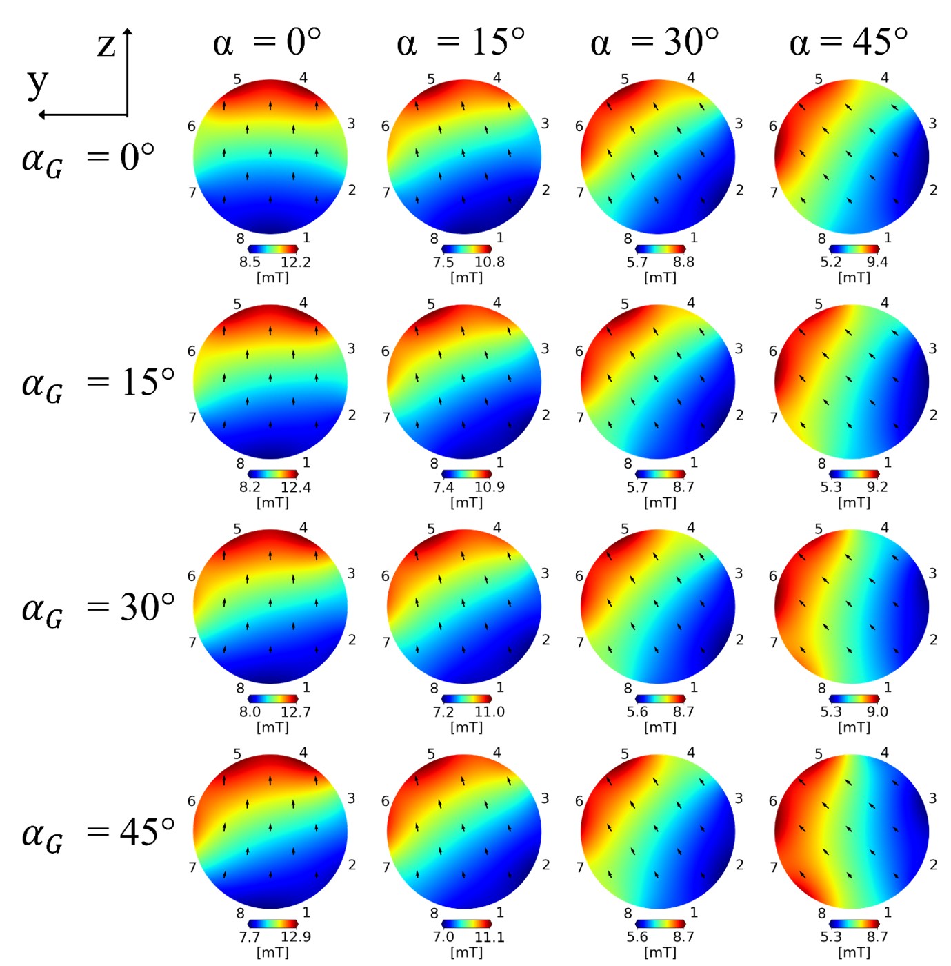
The methods outlined above were applied to an 8×3 loop array (diameter:100mm, length:100mm) to generate a uniform field and 3-axis gradient field within a region of interest (ROI) measuring 50mm in diameter and 50mm in length. The B₀ maps for the 8-element loop array (diameter:100mm, length:100mm) were calculated for various $$$\alpha$$$ values ($$$0^\circ$$$,$$$15^\circ$$$,$$$30^\circ$$$,and $$$45^\circ$$$) and $$$\alpha_g$$$ (angle between main field and gradient field) values ($$$0^\circ$$$,$$$15^\circ$$$,$$$30^\circ$$$,and $$$45^\circ$$$) within the same ROI. All loops were considered as 100-turns with a maximum current of 5A.

Results

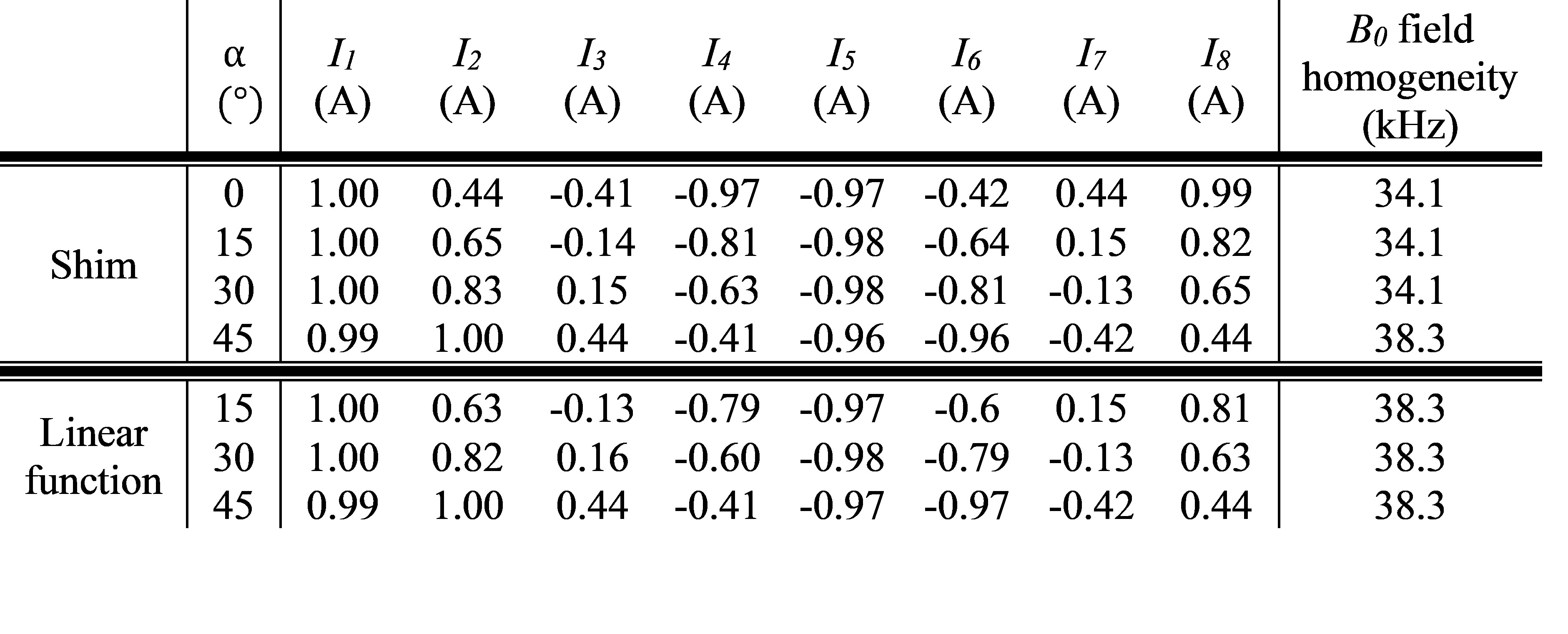
In Figure 2, the calculated magnetic field map of the 24-element array is shown for different modes of the array. The multi-row configuration enables the generation of 3-axis gradient fields, in addition to a uniform field. Thus the array is suitable for spatial encoding in all three directions.
While the fields in Figure 2 show different spatial patterns for B_z component, Figure 3 shows the uniform magnetic field mode generated for different orientations in the yz plane. Table 1 details the individual coil current values for creating a uniform B₀ field and the field uniformity in different directions. Figure 4 illustrates the B₀ field with gradient field suitable for spatial encoding. This figure demonstrates the direction adjustability of not only the main field but also the gradient field in the horizontal plane.

Discussion

We've shown a multi-element array coil's utility for low-field MRI, serving as both the main magnetic and linear gradient field source. The proposed loop coil array achieves uniform magnetic field generation and magnetic field direction control. This approach enables a simplified single-layer configuration of magnet and 3-axis gradient coils that reduces weight and volume. However, since magnetic field uniformity and gradient linearity aren't as optimal as high field MRI system, algebraic reconstruction based on field map measurements becomes essential^4,5.

Conclusions

We've shown that a loop coil array generates uniform magnetic fields via current adjustments, offering directional control and gradient field creation. A method for calculating required current values has been presented, and simulations validate its effectiveness. Such coil arrays can replace traditional magnets and 3-axis gradient coils in low-field MRI, potentially leading to more compact and lighter systems.

Acknowledgements

No acknowledgement found.