2812
Deep Learning-Assisted Joint Estimation for 3D Retrospective Motion Correction: An In-Vivo Validation1BRAIN-To Lab, University Health Network, Toronto, ON, Canada, 2Department of Medical Biophysics, University of Toronto, Toronto, ON, Canada, 3Toronto Neuroimaging Facility, Department of Psychology, University of Toronto, Toronto, ON, Canada
Synopsis
Keywords: Motion Correction, Motion Correction, Neuroimaging, AI
Motivation: Data-driven retrospective motion correction methods currently face challenges with respect to robustness and long runtimes, which can be addressed by combining deep learning- and physics-based methods.
Goal(s): To validate a novel deep learning-assisted joint estimation algorithm on real motion-corrupted 3D MRI data.
Approach: A dataset of motion-corrupted data was acquired on 4 healthy volunteers. The performance of the proposed method was compared to a state-of-the-art deep learning method and a physics-based method.
Results: The proposed method outperformed the deep learning- and physics-based methods, yielding better image correction and converging faster.
Impact: The proposed retrospective motion correction method can be adopted into clinical practice as an alternative to rescanning, having demonstrated that it can salvage real motion-corrupted data without special hardware and requiring minimal sequence modifications.
Introduction
Patient head motion is a common cause of image degradation in MR neuroimaging [1]. Retrospective motion correction (RMC) aims to salvage corrupted data and includes physics-based [2], [3] and deep learning-based [4] methods. Building upon a promising 2D correction approach that combined signal modeling and deep learning [5], in this work we evaluated the performance of a deep learning-assisted algorithm for joint image and 3D motion estimation [6] on real motion-corrupted data.Methods
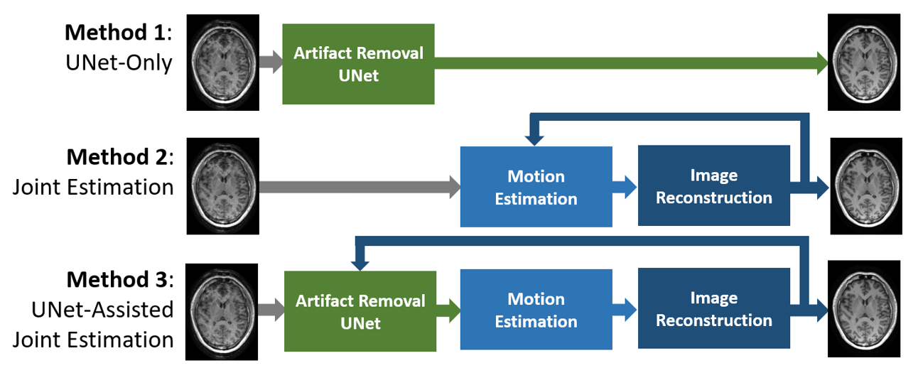
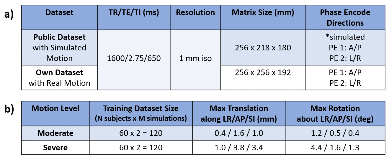
We compared three RMC methods, which are summarized in Fig 1.Method 1 is the Stacked UNet with Self-Assisted Priors [7]. We trained the network on a dataset of simulated moderate and severe motion corruption, which was generated from a public dataset of motion-free T1w MPRAGE complex image data [8]. Please refer to Fig 2a for the scanning parameters and Fig 2b for the training dataset details. We adapted the UNet for complex data by training separate networks for real and imaginary image components.
Method 2 is the 3D joint image and motion estimation algorithm [3], which estimates the motion-free image and motion trajectory by alternately solving Eq 1 and 2:
| | $$$\hat{m}=\arg\min_{m}||E_{\hat\theta}m-s||^2$$$ | (1) |
| | $$$\hat{\theta}=\arg\min_{\theta}||E_{\theta}W\hat{m}-s||^2$$$ | (2) |
where $$$E_\theta$$$ = MRI signal encoding operator [9], $$$m$$$ = magnetization, $$$s$$$ = MRI signal, $$$\theta$$$ = rotation and translation operators, and $$$W$$$ = a binary mask that crops axial slices below the cerebellum. Eq 1 is solved using CG-SENSE [10] and Eq 2 is solved using the BFGS algorithm [11].
The UNet-assisted Joint Estimation algorithm (Method 3) incorporates Method 1 within each iteration of Method 2:
| | $$$\hat{\theta}=\arg\min_{\theta}||E_{\theta}W(UNet(\hat{m}))-s||^2$$$ | (3) |
Experimental Data
T1w MPRAGE data were acquired from 4 healthy participants on a 3T PRISMA Siemens scanner using a 20-channel head array coil. The TR/TE/TI were matched to the public dataset used to train the UNet (Fig 2a). Two motion-corrupted scans and a motion-free ("reference") scan were acquired from each participant. The reference scans were acquired with standard linear phase-encode ordering. The motion-corrupted scans were acquired with an interleaved ordering, whereby the 256 first-phase-encode steps were divided into 16 segments (“shots”); each shot consisted of 16 equidistant TRs, resembling a Cartesian sampling pattern with an effective undersampling factor of R=16.
Image Quality Assessment
We evaluated the performance of the three methods by computing the image percent error (ϵ) and structural similarity index (SSIM). Additionally, we carried out grey matter segmentation using FMRIB’s Automated Segmentation Tool [12] on the motion-corrected images and evaluated Dice coefficients, false-positive rates (FPR) and false-negative rates (FNR). Prior to computing these metrics, the reference scans were rigidly registered [13] to the corresponding image output of each RMC methods and a skull-stripping mask [14] was applied. We assessed image quality improvement by computing the relative change of each metric ($$$\Delta_x=\frac{x_{final}-x_{initial}}{x_{initial}}$$$ for a given metric $$$x$$$).
Results
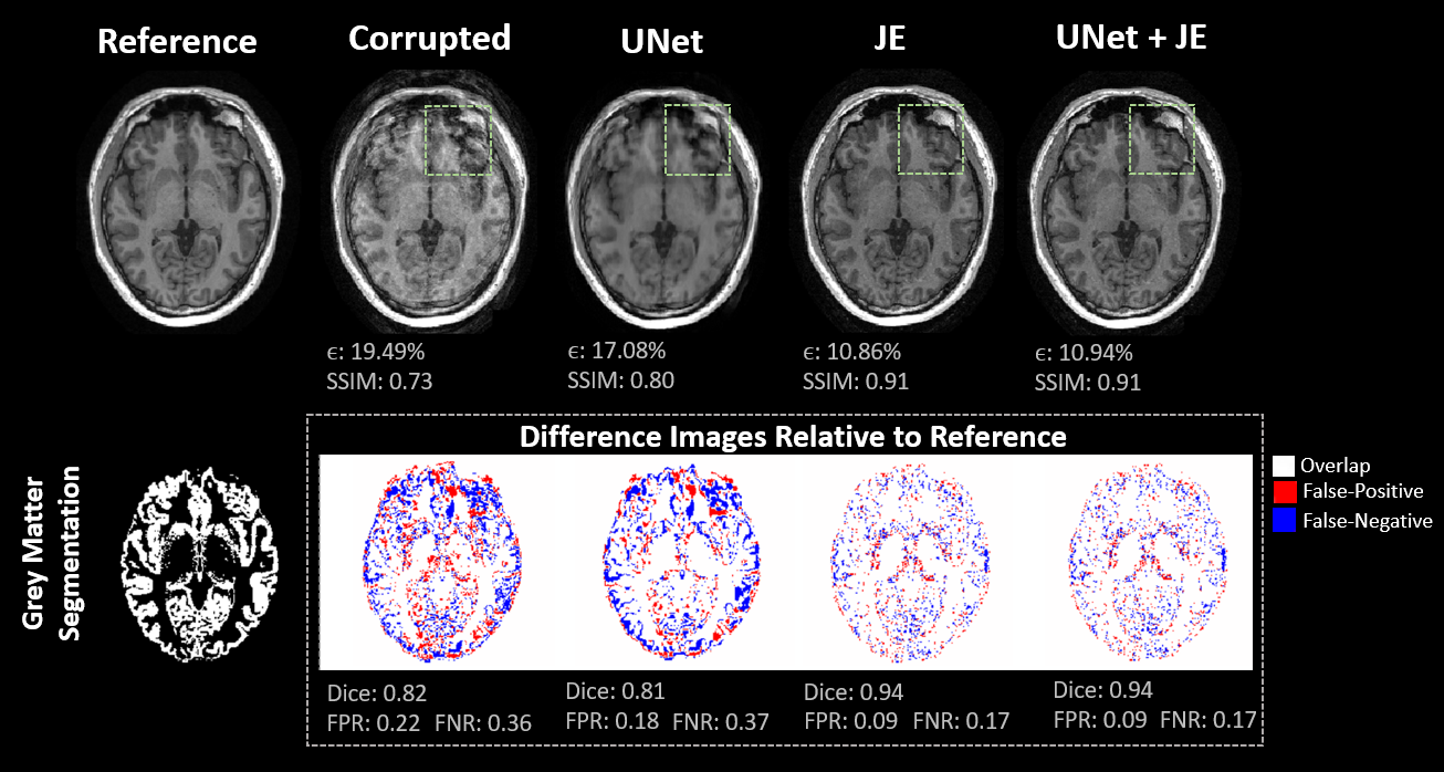
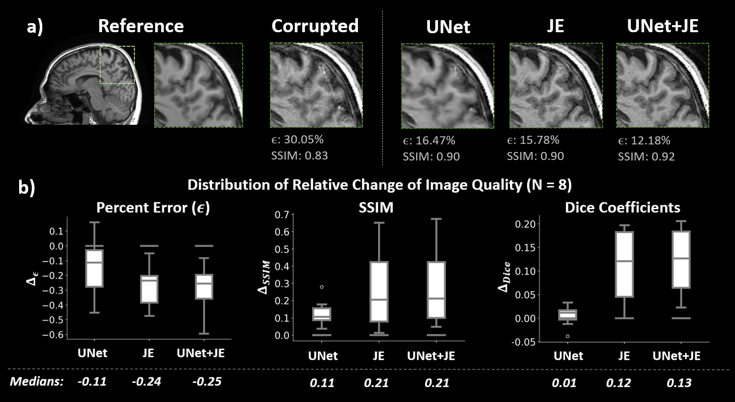
Methods 2 and 3 produced high-quality motion-corrected T1w images, while Method 1 consistently resulted in image blurring. Fig 3 shows a representative case, where the differences in image correction quality are reflected in the false-positive and false-negative rates during grey matter segmentation. When comparing the FPR and FNR across the test dataset, Method 3 had the lowest median $$$\pm$$$ interquartile range (0.12$$$\pm$$$0.04 and 0.21$$$\pm$$$0.04, respectively), while Method 1 had the largest (0.17$$$\pm$$$0.11 and 0.34$$$\pm$$$0.14).While Methods 2 and 3 generally converged to similar images, we found 2 cases where Method 3 converged to better image estimates. Fig 4a demonstrates one such case, highlighting residual artifacts that are present in Method 2 and that are absent in Method 3.
Fig 4b shows the distribution of relative change of $$$\epsilon$$$, SSIM, and Dice coefficients; the FPR and FNR were omitted because they followed similar trends as the Dice coefficients. When comparing the median relative changes (displayed in the bottom row), we found that Methods 2 and 3 similarly outperformed Method 1 across all metrics.
When comparing the runtimes of Methods 2 and 3, we found that the inclusion of the UNet (Method 3) reduced runtimes by a median factor of 2.44 (maximum: 6.31; minimum: 1.55).
Discussion and Conclusions
We validated Method 3 on real motion-corrupted data. We demonstrated that this method outperformed Methods 1 and 2, providing better image correction than the former and converging faster than the latter. Method 3 was also shown to converge to a better image estimate than Method 2 in a few cases. Future work will include implementing intra-shot motion correction and testing Method 3 on clinical data.Acknowledgements
No acknowledgement found.References
[1] M. Zaitsev, J. Maclaren, and M. Herbst, “Motion artifacts in MRI: A complex problem with many partial solutions,” J. Magn. Reson. Imaging, pp. 887–901, Jan. 2015, doi: 10.1002/jmri.24850.
[2] D. Atkinson, D. L. G. Hill, P. N. R. Stoyle, P. E. Summers, and S. F. Keevil, “Automatic correction of motion artifacts in magnetic resonance images using an entropy focus criterion,” IEEE Transactions on Medical Imaging, vol. 16, no. 6, pp. 903–910, Dec. 1997, doi: 10.1109/42.650886.
[3] L. Cordero-grande, E. J. Hughes, J. Hutter, A. N. Price, and J. V. Hajnal, “Three-Dimensional Motion Corrected Sensitivity Encoding Reconstruction for Multi-Shot Multi-Slice MRI : Application to Neonatal Brain Imaging,” vol. 1376, pp. 1365–1376, 2018, doi: 10.1002/mrm.26796.
[4] V. Spieker et al., “Deep Learning for Retrospective Motion Correction in MRI: A Comprehensive Review.” arXiv, May 11, 2023. Accessed: May 16, 2023. [Online]. Available: http://arxiv.org/abs/2305.06739
[5] M. W. Haskell et al., “Network Accelerated Motion Estimation and Reduction (NAMER): Convolutional neural network guided retrospective motion correction using a separable motion model,” Magnetic Resonance in Medicine, vol. 82, no. 4, pp. 1452–1461, 2019, doi: 10.1002/mrm.27771.
[6] B. Nghiem, Z. Wu, L. Kasper, and K. Uludağ, “Stacked UNet-Assisted Joint Estimation for Robust 3D Motion Correction,” in Proc. Intl. Soc. Mag. Reson. Med. 32, Toronto, Canada, 2023.
[7] M. A. Al-masni et al., “Stacked U-Nets with self-assisted priors towards robust correction of rigid motion artifact in brain MRI,” NeuroImage, vol. 259, p. 119411, Oct. 2022, doi: 10.1016/j.neuroimage.2022.119411.
[8] R. Souza et al., “An open, multi-vendor, multi-field-strength brain MR dataset and analysis of publicly available skull stripping methods agreement,” NeuroImage, vol. 170, pp. 482–494, Apr. 2018, doi: 10.1016/j.neuroimage.2017.08.021.
[9] P. G. Batchelor, D. Atkinson, P. Irarrazaval, D. L. G. Hill, J. Hajnal, and D. Larkman, “Matrix Description of General Motion Correction Applied to Multishot Images,” vol. 1280, pp. 1273–1280, 2005, doi: 10.1002/mrm.20656.
[10] K. P. Pruessmann, M. Weiger, M. B. Scheidegger, and P. Boesiger, “SENSE: Sensitivity encoding for fast MRI,” Magn. Reson. Med., vol. 42, no. 5, pp. 952–962, Nov. 1999, doi: 10.1002/(SICI)1522-2594(199911)42:5<952::AID-MRM16>3.0.CO;2-S.
[11] J. Nocedal and S. J. Wright, Numerical optimization, 2nd ed. in Springer series in operations research. New York: Springer, 2006.
[12] Y. Zhang, M. Brady, and S. Smith, “Segmentation of brain MR images through a hidden Markov random field model and the expectation-maximization algorithm,” IEEE Transactions on Medical Imaging, vol. 20, no. 1, pp. 45–57, Jan. 2001, doi: 10.1109/42.906424.
[13] B. B. Avants, N. J. Tustison, G. Song, P. A. Cook, A. Klein, and J. C. Gee, “A reproducible evaluation of ANTs similarity metric performance in brain image registration,” Neuroimage, vol. 54, no. 3, pp. 2033–2044, Feb. 2011, doi: 10.1016/j.neuroimage.2010.09.025.
[14] A. Hoopes, J. S. Mora, A. V. Dalca, B. Fischl, and M. Hoffmann, “SynthStrip: skull-stripping for any brain image,” NeuroImage, vol. 260, p. 119474, Oct. 2022, doi: 10.1016/j.neuroimage.2022.119474.
Figures