2780
Fingerprint Representation of Metabolite Magnetic Resonance Spectroscopy with Deep Learning1National Institute of Mental Health, Bethesda, MD, United States
Synopsis
Keywords: Machine Learning/Artificial Intelligence, Spectroscopy
Motivation: One of the major challenges for spectral fitting is the modeling of background signals.
Goal(s): Develop a deep learning model for quantitative detection of in vivo metabolites without relying on spectral fitting.
Approach: Spectral fingerprint representation is achieved by combining manifold learning and representation learning, with the tasks that include predicting metabolite concentrations, transverse relaxation times, and reconstructing individual metabolite signals.
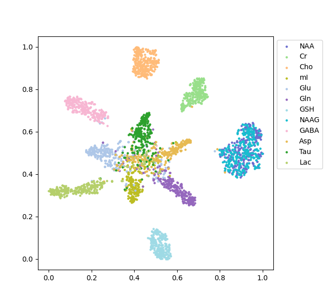
Results: The t-SNE map illustrates that metabolites can be clustered based on the fingerprints generated by the model. The predicted metabolite concentrations and relaxation T2s agree with those found in the literature. The spectral background or unregistered signals are effectively filtered out.
Impact: The deep learning model demonstrates high practical viability for the quantification of metabolite concentrations and relaxation T2s. It essentially searches for learned spectral fingerprints instead of relying on spectral fitting, the latter involves modeling all signals contained in the data.
Introduction
A recently introduced deep learning model directly quantifies metabolite concentrations without relying on spectral fitting1. That model is designed for the dual-task of predicting individual metabolite signals and concentrations simultaneously. It takes time-domain JPRESS data as its input, capitalizing on the wealth information present in a diverse range of spectra with varying echo times. In this abstract, we refine the model proposed in ref. 1 and extend the spectral representation to include, for the first time, the prediction of transverse relaxation time T2. We refer to this extended spectral representation as spectral fingerprint representation and report in vivo test results.Methods
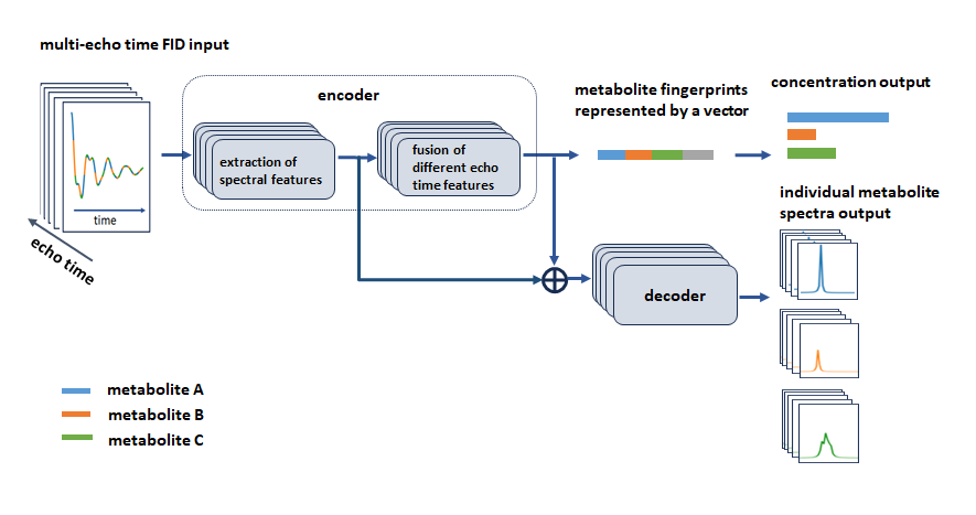
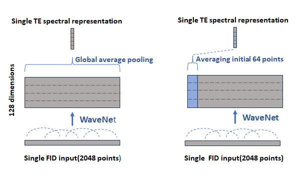
Figure 1 illustrates the forward computation flow of the model for three symbolic metabolites. Commencing with the input of 32-echo Free Induction Decay (FID) signals of JPRESS in the time domain, the model utilizes convolutional WaveNet units to extract target spectral features independently from all input FIDs, generating individual TE spectral representations by averaging the initial 64 points in the sampling dimension, instead of pooling over all sampling points1. Figure 2 illustrates the difference between the two pooling strategies. The new strategy attempts to minimize the interaction between metabolite concentrations and spectral lineshapes. The representations specific to individual echo times are then fused using the Gated Recurrent Unit (GRU) to establish cross-correlations between different echo times to enhance the individual representations, a scheme for aggregating variants that differs from arithmetic averaging. This process block repeats four times, and the resulting TE-specific representations are subsequently averaged to generate the final representation. This final representation captures the essential spectral features of target metabolites and ignores undesired features such as background signals and spectral lineshapes, forming metabolite fingerprints that enable the differentiation of metabolites and directly mapping FIDs to the concentrations and T2s. Furthermore, the model is trained to be phase and frequency-offset invariant.Results and Discussion
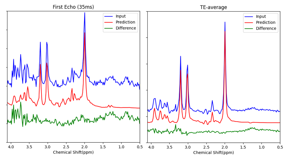
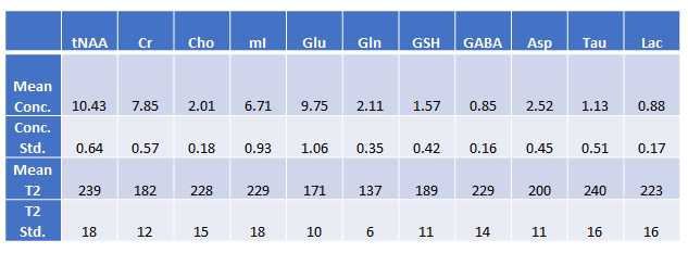
Figure 3 depicts the fingerprints of 12 metabolites visualized with a t-distributed Stochastic Neighbor embedding (t-SNE) map generated with 3200 simulated data sets. Note that NAA and NAAG were combined into a single target during the training and, hence, are indistinguishable. This map illustrates how metabolites can be clustered based on the fingerprints generated by the model. Figure 4 shows an in vivo example for predicting the first echo spectrum and the spectrum averaged from all 32 echoes as compared with the corresponding input spectra. The predicted spectra are obtained by summing all predicted individual component FIDs, including the residual water signal. The difference lines are the residuals of the subtraction of the prediction from the input. Despite the strong spike artifacts in the down-field end of the first echo spectrum, induced by the outer-volume suppression crusher gradients, the model is able to sort out the target signals. The difference residuals for the TE-averaged spectrum features unidentified peaks between 3 and 3.5 ppm. The small “blip” near 3.6 ppm, aligned with the mI peaks on the right, should be attributed to glycine, which is not registered. Table 1 lists the predicted metabolite concentrations and the T2 values for 20 data sets acquired from the healthy brain. The predicted concentrations agree with the literature 2-4, and the T2 predictions are generally within the ranges reported in the literature 5-7.Global average pooling generates a TE-specific spectral representation akin to the area integral of spectral peaks. In contrast, averaging the initial 64 sampling points is more related to using the signal amplitudes for representing concentrations. Our new approach leads to closer and more consistent agreement between the predicted metabolite concentration and FIDs, which has been observed in our validation results. WaveNet establishes short- and long-range spectral feature correlations through convolutional operations. Ideally, a single first point should be able to capture the entire echo spectral features with the WaveNet operation and yield metabolite concentrations without the influence of spectral lineshapes. However, in the current model, the dilation depth of the WaveNet is optimally set at 8, corresponding to a maximum correlation distance of 256 points. As a result, using too few data points cannot resolve metabolite components due to significant information loss. On the other hand, our experiments show that, using a deeper dilation depth, consequently with longer correlation distances, can lead to overfitting rather than improving model performance.
Conclusion
The proposed deep learning model demonstrates high practical viability. It essentially searches for learned spectral fingerprints, instead of relying on fitting using model spectra. This deep learning approach opens up opportunities for the non-invasive quantitative detection of low-concentration metabolites with improved accuracy.Acknowledgements
No acknowledgement found.References
1. Zhang Y and Shen J. Quantification of spatially localized MRS by a novel deep learning approach without spectral fitting. Magn Reson Med. 2023; 90:1282-1296.
2. Penner J and Robert BR. Semi-LASER 1 H MR spectroscopy at 7 tesla in human brain: metabolite quantification incorporating subject-specific macromolecule removal. Magn Reason Med. 2015; 74: 4-12. 3. Deelchand DK, et al. Improved localization, spectral quality, and repeatability with advanced MRS methodology in the clinical setting. Magn Reson Med. 2017; 79: 1241-1250.
4. Marjańska M, et al. Localized 1H NMR spectroscopy in different regions of human brain in vivo at 7T: T2 relaxation times and concentrations of cerebral metabolites. NMR Biomed. 2012; 25: 332-339. 5. Ganjia SK, et al. T2 measurement of J-coupled metabolites in the human brain at 3T. NMR Biomed. 2012; 25: 523-529.
6. Traber F, et al. 1H metabolite relaxation times at 3.0 tesla: Measurements of T1 and T2 values in normal brain and determination of regional differences in transverse relaxation. J Magn Reson Imaging. 2004; 19:537-545.
7. Zaaraoui W, et al. Human brain-structure resolved T2 relaxation times of proton metabolites at 3 Tesla. Magn Reson Med. 2007; 57:983-989.
Figures