2749
Renal Mesh to Perform Regional Perfusion Analysis of The Kidney1Department of Radiology and Nuclear Medicine, Ghent University Hospital, Gent, Belgium, 2Department of Diagnostic Sciences, Faculty of Medicine and Health Sciences, Ghent University, Gent, Belgium, 3Ghent Institute of Functional and Metabolic Imaging (GIFMI), Ghent University, Gent, Belgium, 4IBiTech– Medisip, Ghent University, Gent, Belgium
Synopsis
Keywords: Kidney, Kidney
Motivation: ASL-measured perfusion values are assumed to change homogeneously across the kidney. We believe that additional information might be retrieved by analyzing regional perfusion differences.
Goal(s): Renal perfusion is assumed to decrease with aging but also in renal pathologies.
- Does renal perfusion decrease uniformly?
Approach:
- Retrieve renal ASL images from 27 subjects.
- Create one 2D mesh per subject.
- Pool the results for 3 different groups.
- Analyze the variation of renal perfusion.
Results:
- Patients compared to younger healthy volunteers (HVs) show lower perfusion.
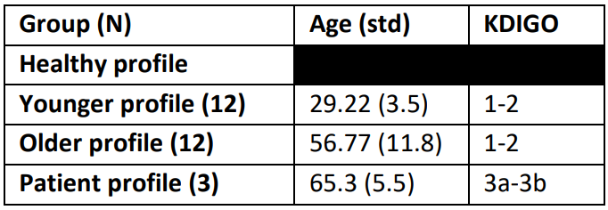
- Patients compared to older HVs exhibit a negative variation in the kidney lateral outermost region, while other regions show higher perfusion values.
Impact: Understanding kidney blood flow patterns could aid early disease detection and personalized treatments. Identifying specific regions affected in kidney patients might improve targeted therapies. This knowledge may enhance patient outcomes, potentially leading to a better life quality for kidney patients.
Introduction
Renal arterial spin labeling (ASL) stands out as a promising technique in magnetic resonance imaging (MRI). Consensus literature indicates that Renal ASL measures higher perfusion values in the cortex and lower values in the medulla1,2,3. Previous phases of this study showed that perfusion diminishes from the kidney's outer regions toward the inner regions4. Moreover, higher perfusion values are seen in the lateral regions of the kidney than in the upper and lower poles4. The goal of this study was to create a 2D mesh to analyze how the perfusion changes regionally, in both directions radially and, from the lower pole to the upper pole.Methods
The renal mesh $$$V_{\text{grid}}(i,j)$$$ (Fig 2b) is a two-dimensional (2D) grid that is divided into regions ($$$Regions=Sections\cdot Layers $$$) where Sections represent the number of equiangular objects (EO)4. Layers represent the number of concentric objects (CO)5. These were the steps to create the renal mesh $$$V_{\text{grid}}(i,j)$$$:- Slice Definition: a coronal slice was defined from a volumetric ASL image.
- Kidney Masking: draw a binary mask for the kidney image $$$V_{\text{binary}}(i,j)$$$, (Fig.1a).
- Algorithm Application: Apply the CO and EO algorithms to $$$V_{\text{binary}}(i,j)$$$, to obtain the $$$V_{\text{EO}}(i,j)$$$ and $$$V_{\text{CO}}(i,j)$$$, (Fig.1a and Fig.1b).
- Table Creation: set up a table $$$T$$$, with a number of rows ($$$n_{\text{row}}=Sections$$$) and number of columns ($$$n_{\text{column}}=Layers$$$). The table $$$T$$$ is filled with the numbers ranging from 1 to the total regions (Fig.2a).
- Iterative Process: Iterate over the length and width of $$$V_{\text{binary}}(i,j)$$$, $$$V_{\text{EO}}(i,j)$$$ and $$$V_{\text{CO}}(i,j)$$$ masks, for the pixels where $$$V_{\text{binary}}(i,j)=1$$$, (Fig.1a)
- 5.a Read the value of $$$V_{\text{EO}}(i,j)=a$$$ at the given point (Fig.1b).
- 5.b Read the value of $$$V_{\text{CO}}(i,j)=b$$$ at the given point (Fig.1c).
- 5.c Read the value of the table $$$T$$$ at the column b and row a. So $$$V_{\text{2d}}(i,j)=T(a,b)$$$
- 5.d Assign the value $$$V_{\text{2d}}$$$ to the mesh mask, $$$V_{\text{grid}}(i,j)=V_{\text{2d}}$$$, (Fig 2b).
Results
In each subject, a kidney grid was generated (Fig.1 and Fig.2). The mean perfusion values for each region were calculated. Healthy profiles (HP) were obtained by averaging the perfusion values within each region across subjects. The younger HP displayed perfusion rates ranging from 96-176 ml/min/100g (Fig.3: 1a and 1b), while the older HP exhibited values between 53-110 ml/min/100g (Fig.3: 2a and 2b). Patients' profiles reported perfusion values from 62-107 ml/min/100g (Fig 3a and 3b).Analyzing the percentage change between the younger group and the patient group revealed a decrease in perfusion values ranging from -14% to -49% (Fig.4: a and b). Similarly, when comparing the older group with the patient group, differences in perfusion values were observed, ranging from -15% to 29% (Fig 4: c and d).
Discussion
Regional changes in renal perfusion have been discussed in the literature. It has been shown that perfusion values in the renal cortex are higher than in the medulla1,2,3. It's been noted that CKD patients show lower perfusion values1,3 in the renal cortex. Our study aligns with these findings, demonstrating consistently lower perfusion values in patients compared to younger HVs across the entire kidney. Interestingly, when comparing patients to older HVs, it becomes evident that the negative variation primarily occurs in the lateral outermost region of the kidney. Conversely, both the lower and upper poles exhibit higher values in patients compared to older HVs. This suggests a potential focal impact on the lateral renal cortex in patients classified between KDIGO 3a and 3b. However, it is essential to expand the study to a more diverse population, including a wider range of ages and KDIGO classifications, to validate these preliminary results.Conclusion
Renal perfusion has been evaluated as the mean value of the whole kidney or the mean value of regions of interest in the cortex and medulla. The use of renal mesh confirms that there are regional changes in kidney perfusion. The Histological investigation would be useful to validate the results obtained here. By changing the number of layers or sections, an optimal configuration may be found depending on the application.Acknowledgements
The authors thank Dr. Bernd Kühn (Siemens Healthcare AG, Erlangen, DE) for providing the ASL WIP sequence.References
- Cox EF, Buchanan CE, Bradley CR, Prestwich B, Mahmoud H, Taal M, et al. Multiparametric Renal Magnetic Resonance Imaging: Validation, Interventions, and Alterations in Chronic Kidney Disease. Frontiers in physiology 2017;8:696.
- Eckerbom P, Hansell P, Cox E, Buchanan C, Weis J, Palm F, Francis S, Liss P. Multiparametric assessment of renal physiology in healthy volunteers using noninvasive magnetic resonance imaging. Am J Physiol Renal Physiol. 2019 Apr 1;316(4):F693-F702. doi: 10.1152/ajprenal.00486.2018. Epub 2019 Jan 16. PMID: 30648907.
- Buchanan CE, Mahmoud H, Cox EF, McCulloch T, Prestwich BL, Taal MW, Selby NM, Francis ST. Quantitative assessment of renal structural and functional changes in chronic kidney disease using multi-parametric magnetic resonance imaging. Nephrol Dial Transplant. 2020 Jun 1;35(6):955-964. doi: 10.1093/ndt/gfz129. PMID: 31257440; PMCID: PMC7282828.
- Sanmiguel LC, De Visschere P, Speeckaert M, Pullens P. A NEW METHOD TO ANALYSE RENAL PERFUSION: A PROOF OF CONCEPT, 2023 ISMRM Annual Congress Toronto
- Piskunowicz M, Hofmann L, Zuercher E, Bassi I, Milani B, Stuber M, et al. A new technique with high reproducibility to estimate renal oxygenation using BOLD-MRI in chronic kidney disease. Magnetic resonance imaging 2015 Apr;33:253–61.
Figures
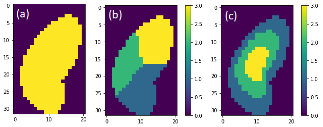
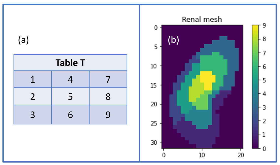
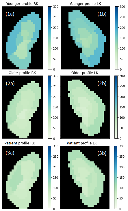
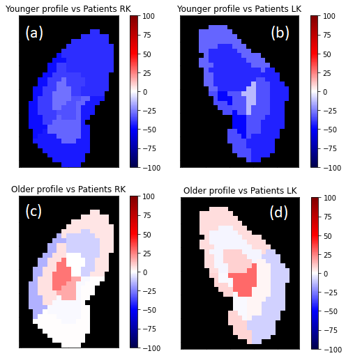
Figure. 4 Percentage of change of patient profile with respect to the healthy mesh. Compared to younger profile (a) Right kidney, (b) Left kidney. Compared to older profile, (c) Right kidney and (d) Left kidney. Color bar scale in percentage [%].