2748
Volumetric Layer Based Analysis for Quantitative Renal MRI1Sir Peter Mansfield Imaging Centre, University of Nottingham, Nottingham, United Kingdom
Synopsis
Keywords: Kidney, Data Analysis, Layers
Motivation: To provide improved methods to estimate cortical-medullary changes in multiparametric MRI measures of the kidney.
Goal(s): To develop an analysis method for use with 3D data to generate quantitative-depth-based cortical-medullary layers which can be applied to any multiparametric map.
Approach: 3DQLayers segments the kidney into layers based on their distance from the renal surface using the Trimesh Python library.
Results: Generated 3D layers can be applied to multiparametric MRI scans collected in the same session. Here, this is applied to assess cortical layer profiles and contour plots of quantitative T1-mapping, R2*-mapping and perfusion measures, and to estimate renal cortical thickness.
Impact: 3DQLayers provides a layer-based analysis technique for renal multiparametric MRI data, extending traditional ROI-based methods. Layer profiles of any quantitative MRI data can be output and average renal cortical thickness estimated, these are important measures to study in renal disease.
Introduction
Key to the analysis of renal MRI studies is the reporting of quantitative measures in the cortex and medulla. This is often performed using manual regions-of-interest (ROI) which are difficult to define, whilst automated methods of segmenting the kidney using thresholding1 or machine learning2 are being developed. The twelve layer concentric object (TLCO) method was proposed by Pruijm et al3–6 as an alternative to ROI analysis when studying BOLD R2* maps. This method uses two user-delineated boundaries to generate twelve equidistant layers between the renal pelvis and surface, the average R2* in each layer is calculated, from which R2*outer, R2*inner, and R2*slope, representing cortex, medulla and cortico-medullary difference is computed. TLCO uses a single slice, coronal oblique acquisition. However the BOLD consensus survey7, highlighted the need for oblique coronal images for TLCO, which was not always the preferred acquisition. This and the limitation of a single slice acquisition for TLCO were the motivation for 3DQLayers, a 3D quantitative-depth-based method.Methods
3DQLayers generates renal layers from a whole-kidney structural, here from a T2-weighted FSE scan, that is automatically segmented using a U-Net8,9. The layers are then applied to quantitative data collected in the same scan session, here those collected using the UKRIN-MAPS10,11 protocol.Generating Layers: Layer analysis is performed using the Trimesh package12 in Python. First, a binary kidney mask is generated, Figure 1ai and any holes resulting from cysts are filled, Figure 1aii. The kidney mask is converted from a voxel-representation to a surface-mesh-representation using the marching cubes algorithm13, Figure 1bi. Since renal acquisitions tend to have a higher in-plane than through-plane resolution, mutable diffusion Laplacian smoothing is applied to the mesh14, Figure 1bii. Next, the distance from the centre of each voxel in the kidney mask to the mesh surface is calculated, producing a depth map, Figure 1biii. As the tissue adjacent to the renal pelvis is not representative of medulla, this is automatically excluded from the resulting depth map. First, the pelvis is automatically segmented, Figure 1ci, and the distance from each voxel in the kidney to the pelvis calculated as above, Figure 1cii. Voxels closer than a specified threshold, typically 10mm, are excluded from the depth map, Figure 1ciii. Finally, a layer image is generated by quantising the depth map to a desired layer thickness, typically 1mm, Figure 1d.
Applying Layers to Quantitative Data: The layers are then resampled using NiBabel15 to the same space as the quantitative maps, here to exemplify the method T1-weighted images, MOLLI T1-mapping, and ASL images are used. Voxel-wise measures within each layer (median or histogram mode) along with the gradient of each measure as a function of depth (as in Pruijm et al5,6) are calculated. Cortical/medullary masks generated from the T1-mapping data (FSL topup16,17, FSL FAST18 and manually correction) are used to label the layers.
Results
Figure 2 shows the application of 3DQLayers to T1-weighted, MOLLI T1-mapping, and ASL perfusion-weighted images and the associated layer profile and contour plots. T1-weighted data shows decreasing intensity as a function of layer depth. The contour plot verifies the medulla located deeper in the kidney has generally lower signal, and cortical tissue is mostly found near the surface and deeper surrounding the medullary pyramids. Greater contrast is seen between cortex and medulla for the T1-map, with the contour plot showing two distinct clusters separated by T1 and depth. Figure 3 shows 3DQLayers applied to BOLD R2* maps, with a decreased R2*slope in disease compared to a healthy subject. In Figure 4, by using cortex and medulla mask labels, the layer analysis provides a measure of average cortical thickness.Discussion
The 3DQLayers method decouples layer generation from the quantitative map being studied, increasing flexibility for investigators, one of the concerns with TLCO. Additionally, by defining layers from a whole kidney image, the layer dimensions are quantitative (in mm rather than layer number), thus any derived parameters control for kidney size which changes with renal health19,20. Further, by generating 3D layers for the whole kidney the number of voxels interrogated in the quantitative map is increased, allowing more/thinner layers to be used. The decrease in R2*slope in CKD subjects observed by Pruijm et al6 using TLCO was seen using 3DQLayers. Finally, if cortex/medulla ROIs are generated, the depth map can be used to calculate cortical thickness, a potential biomarker21.Conclusion
3DQLayers can be used to assess layer profiles and contour features in quantitative renal multiparametric MRI data in health and disease. If cortical/medullary ROI are available, 3DQLayers can be used to compute average cortical thickness.Acknowledgements
The authors thank UKRIN-MAPS for the use of their acquisition protocol.References
1. Cox EF, Buchanan CE, Bradley CR, et al. Multiparametric Renal Magnetic Resonance Imaging: Validation, Interventions, and Alterations in Chronic Kidney Disease. Front Physiol. 2017;8:696. doi:doi:10.3389/fphys.2017.00696
2. Eleanor Cox, Zhendi Gong, Martin Craig, et al. Automated Analysis of Kidney MRI data in the UK Biobank. In: Fifth International Renal Imaging Meeting. Ghent, Belgium; 2023.
3. Piskunowicz M, Hofmann L, Zuercher E, et al. A new technique with high reproducibility to estimate renal oxygenation using BOLD-MRI in chronic kidney disease. Magn Reson Imaging. 2015;33(3):253-261. doi:10.1016/j.mri.2014.12.002
4. Milani B, Ansaloni A, Sousa-Guimaraes S, et al. Reduction of cortical oxygenation in chronic kidney disease: evidence obtained with a new analysis method of blood oxygenation level-dependent magnetic resonance imaging. Nephrol Dial Transplant. 2017;32(12):2097-2105. doi:10.1093/ndt/gfw362
5. Pruijm M, Milani B, Pivin E, et al. Reduced cortical oxygenation predicts a progressive decline of renal function in patients with chronic kidney disease. Kidney Int. 2018;93(4):932-940. doi:10.1016/j.kint.2017.10.020
6. Li LP, Milani B, Pruijm M, et al. Renal BOLD MRI in patients with chronic kidney disease: comparison of the semi-automated twelve layer concentric objects (TLCO) and manual ROI methods. Magn Reson Mater Phys Biol Med. 2020;33(1):113-120. doi:10.1007/s10334-019-00808-5
7. Bane O, Mendichovszky IA, Milani B, et al. Consensus-based technical recommendations for clinical translation of renal BOLD MRI. Magn Reson Mater Phys Biol Med. 2020;33(1):199-215. doi:10.1007/s10334-019-00802-x
8. Will S, Martirosian P, Würslin C, Schick F. Automated segmentation and volumetric analysis of renal cortex, medulla, and pelvis based on non-contrast-enhanced T1- and T2-weighted MR images. Magn Reson Mater Phys Biol Med. 2014;27(5):445-454. doi:10.1007/s10334-014-0429-4
9. Daniel AJ, Buchanan CE, Allcock T, et al. Automated renal segmentation in healthy and chronic kidney disease subjects using a convolutional neural network. Magn Reson Med. 2021;86(2):1125-1136. doi:https://doi.org/10.1002/mrm.28768
10. Buchanan CE, Li H, Nery F, et al. Harmonisation of Multiparametric Renal MRI for Multi-Centre Studies. In: Proc. Intl. Soc. Mag. Reson. Med. 29. Vol 29. Online; 2021:0417.
11. UK Renal Imaging Network (UKRIN): MRI Acquisition and Processing Standardisation (MAPS). https://www.nottingham.ac.uk/research/groups/spmic/research/uk-renal-imaging-network/ukrin-maps.aspx. Accessed July 10, 2023.
12. Dawson-Haggerty M. Trimesh. October 2023. https://github.com/mikedh/trimesh. Accessed October 26, 2023.
13. Lorensen WE, Cline HE. Marching cubes: A high resolution 3D surface construction algorithm. ACM SIGGRAPH Comput Graph. 1987;21(4):163-169. doi:10.1145/37402.37422
14. Barroqueiro B, Andrade-Campos A, Dias-de-Oliveira J, Valente RAF. Bridging Between Topology Optimization and Additive Manufacturing via Laplacian Smoothing. J Mech Des. 2021;143(091703). doi:10.1115/1.4049864
15. Brett M, Markiewicz CJ, Hanke M, et al. NiBabel. April 2023. doi:10.5281/zenodo.591597
16. Andersson JLR, Skare S, Ashburner J. How to correct susceptibility distortions in spin-echo echo-planar images: application to diffusion tensor imaging. NeuroImage. 2003;20(2):870-888. doi:10.1016/S1053-8119(03)00336-7
17. Smith SM, Jenkinson M, Woolrich MW, et al. Advances in functional and structural MR image analysis and implementation as FSL. NeuroImage. 2004;23:S208-S219. doi:10.1016/j.neuroimage.2004.07.051
18. Zhang Y, Brady M, Smith S. Segmentation of brain MR images through a hidden Markov random field model and the expectation-maximization algorithm. IEEE Trans Med Imaging. 2001;20(1):45-57. doi:10.1109/42.906424
19. Buchanan CE, Mahmoud H, Cox EF, et al. Quantitative assessment of renal structural and functional changes in chronic kidney disease using multi-parametric magnetic resonance imaging. Nephrol Dial Transplant. 2019;35(6):955-964. doi:10.1093/ndt/gfz129
20. Gong IH, Hwang J, Choi DK, et al. Relationship Among Total Kidney Volume, Renal Function and Age. J Urol. 2012;187(1):344-349. doi:10.1016/j.juro.2011.09.005
21. Yamashita SR, Atzingen AC von, Iared W, et al. Value of renal cortical thickness as a predictor of renal function impairment in chronic renal disease patients. Radiol Bras. 2015;48(1):12. doi:10.1590/0100-3984.2014.0008
Figures
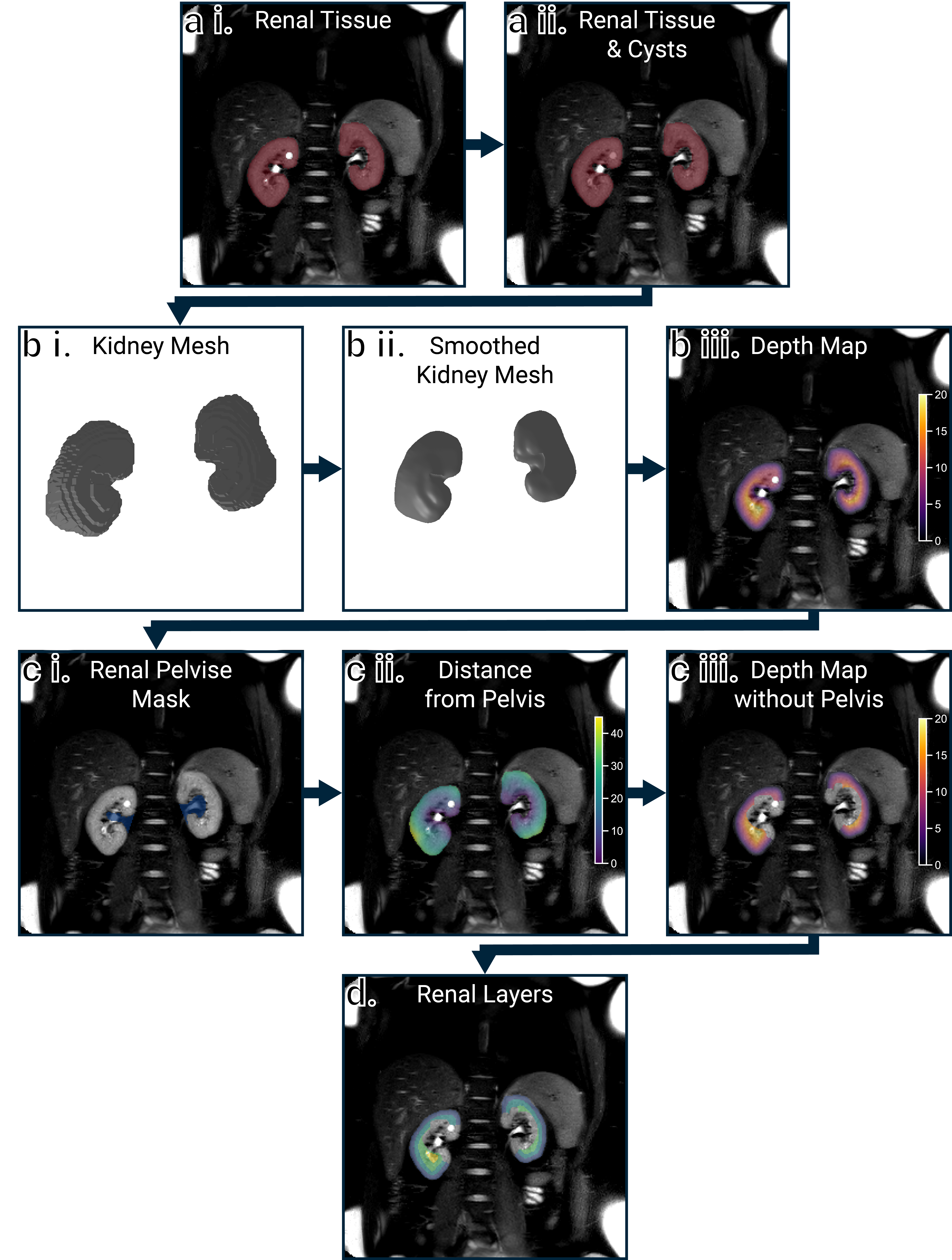
Figure 1: The mask from the T2-weighted FSE scan (a i) has any cysts filled (a ii) and is converted into a smooth mesh representing the renal surface (b i and ii). The distance (in mm) from each voxel to the surface of the mesh is calculated (b iii). The renal pelvis is segmented (c i) and any tissue within 10 mm (c ii) of the pelvis is excluded from the depth map (c iii). The tissue is then grouped into layers of a desired thickness, here shown as 5 mm layers for illustrative purposes (d).
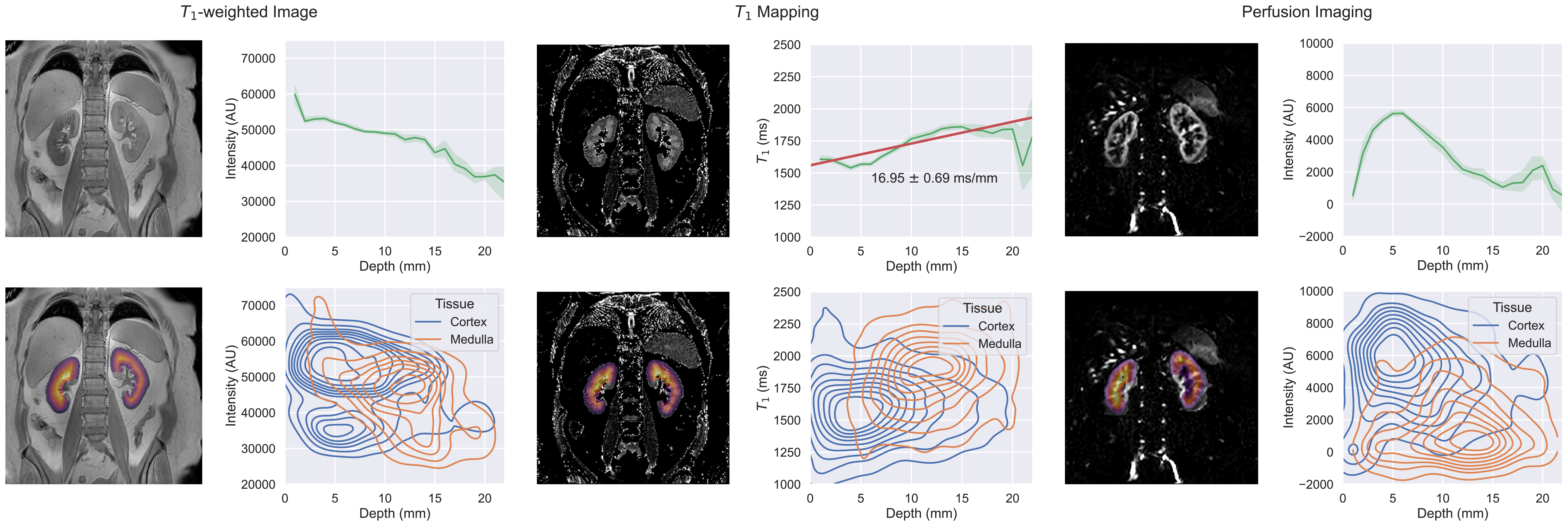
Figure 2: Application of 3DQLayers to T1-weighted data, MOLLI T1-mapping data and ASL perfusion data. Each panel shows the data, the generated layers, a profile of the median parameter in each layer and a contour plot showing how each parameter varies with depth and tissue, with measures including both kidneys. 95% confidence bounds are shown on the line profiles. The T1-mapping contour plot shows better separation between cortex and medulla than for the T1-weighted image due to the influence of B1 causing different signal intensity between the left and right kidney.
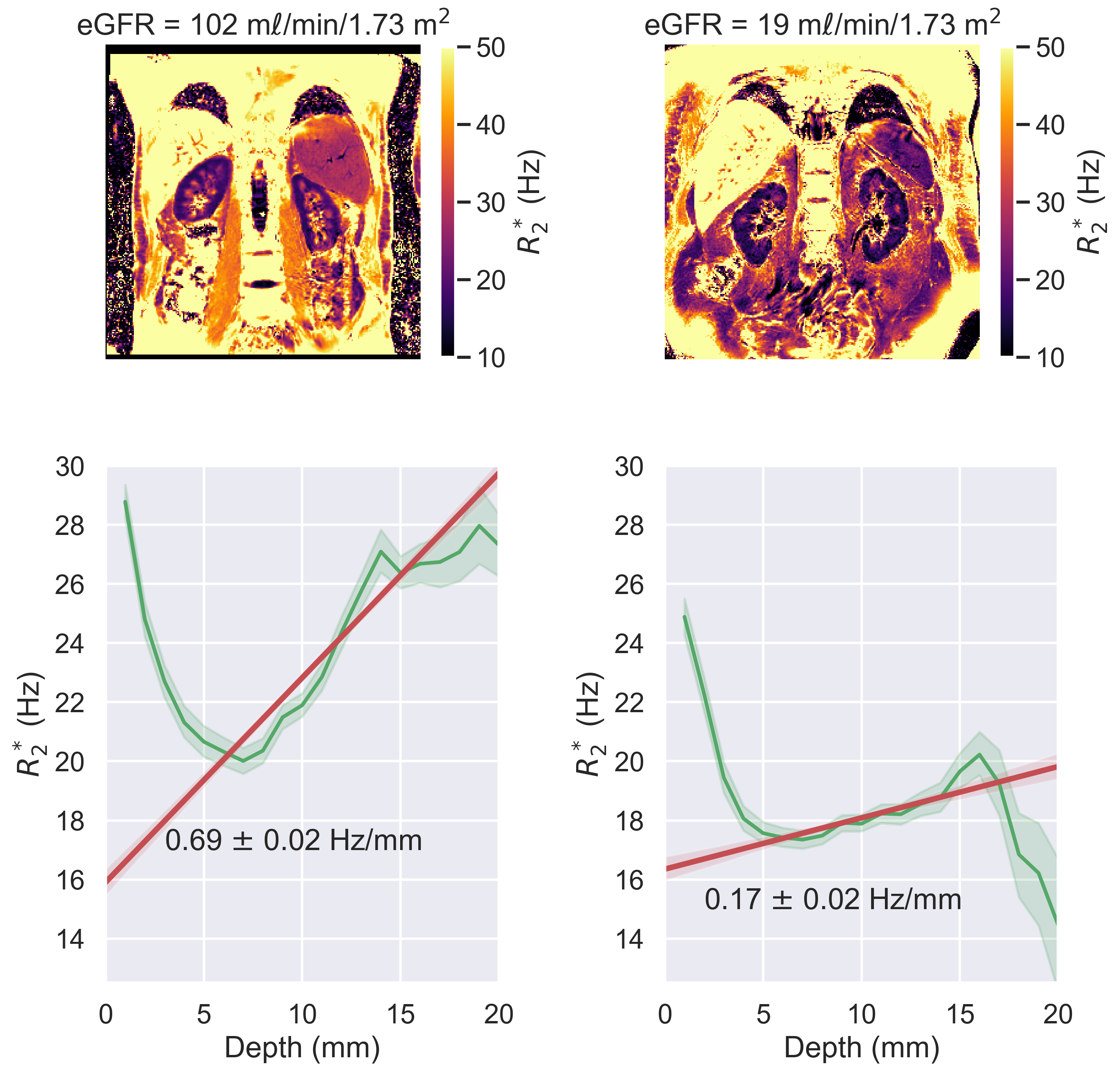
Figure 3: R2* maps and layer profiles for a subject with healthy estimated glomerular filtration rate (eGFR) and low eGFR. 95% confidence bounds are shown on both the line profiles and linear fit. The R2*slope of the centre of the profile is lower in the low eGFR subject as has been shown using TLCO analysis.
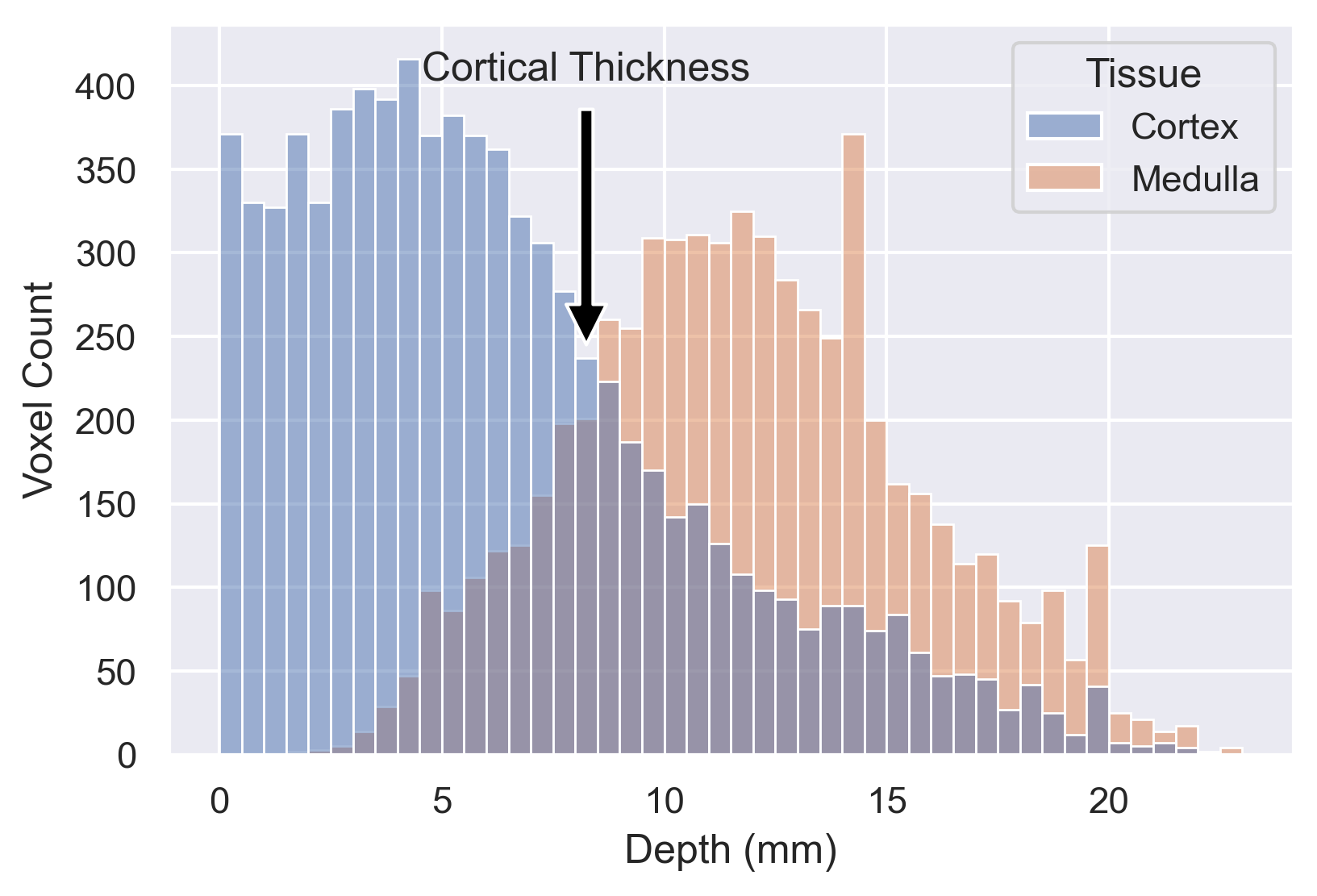
Figure 4: Histogram of number of voxels at each depth in the kidney labelled as cortex and medulla from the masks. From this, the average cortical thickness can be measured, here defined to be the depth at which most renal volume is composed of medullary rather than cortical tissue. Tissue labels generated from T1-mapping data.