2710
A Time-Resolved Forward Model for MR-ARFI: Towards Acoustic Dosimetry for FUS Neuromodulation1Biomedical Engineering, Case Western Reserve University, Cleveland, OH, United States, 2Vanderbilt University, Nashville, TN, United States, 3Radiology, Vanderbilt University, Nashville, TN, United States
Synopsis
Keywords: MR-Guided Focused Ultrasound, Focused Ultrasound, neuromodulation
Motivation: MR-ARFI is currently used to target focused ultrasound in the brain, but as a quantitative imaging method it has the potential to provide acoustic dosimetry if the measured tissue displacement can be related back to acoustic intensity or pressure.
Goal(s): Develop a method to calculate MR-ARFI images based on high-intensity acoustic simulations of focused ultrasound and finite element modeling.
Approach: We converted acoustic beam simulations to acoustic force, which was input to an FEM solver to calculate time-resolved tissue displacements, and subsequently MR-ARFI images.
Results: The method enabled a lookup table calculation to recover acoustic intensity from MR-ARFI measurements
Impact: MR-ARFI is used to target focused ultrasound in the brain, but as a quantitative imaging method it could also provide dosimetry. We established the ability to relate simulated acoustic pressure fields to MR-ARFI images via finite element modeling.
Introduction
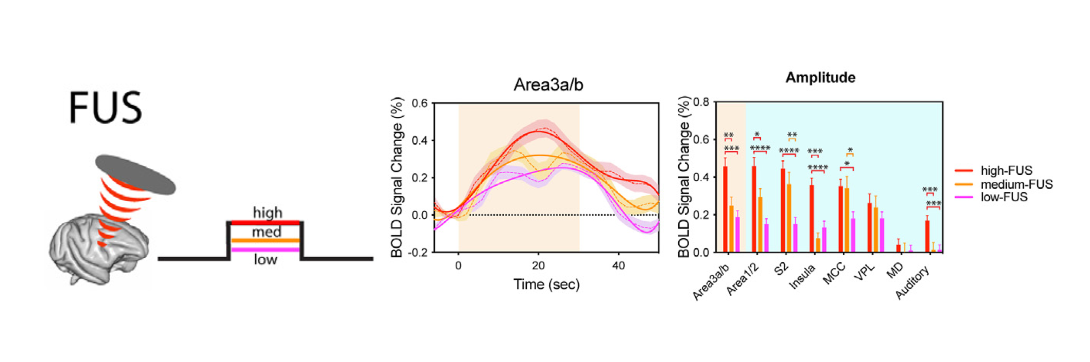
The acoustic radiation force (ARF) applied by focused ultrasound (FUS) causes neuromodulation in the brain, and the level, and type of neuromodulatory effect changes depending on the pressure of the sound wave (Figure 1). Currently, MR-ARFI (Acoustic-Radiation-Force-Imaging) is used to image displacement due to the ARF1 in order to localize the FUS beam2, but the displacement amplitudes have the potential to provide acoustic dosimetry needed to predict neuromodulatory effects, if they can be related back to acoustic intensity or pressure. This requires a forward model relating pressure to MR-ARFI displacement. A method to predict the amount of displacement at steady state has been proposed based on the use of ultrasound pulses long enough (several ms long) to reach steady-state; however, it is desirable to use short ARF pulses in MR-ARFI to minimize bioeffects, which can break the steady state assumption and lead to errors 2. We report a comprehensive forward model to calculate the expected displacement map measured by MR-ARFI, which could enable recovery of acoustic intensity from imaged displacements via, e.g., a lookup table method. This enables the use of MR-ARFI for dosimetry in FUS neuromodulation.Methods
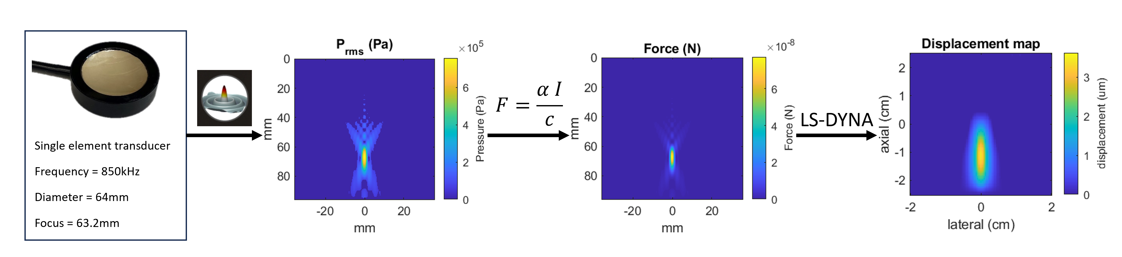
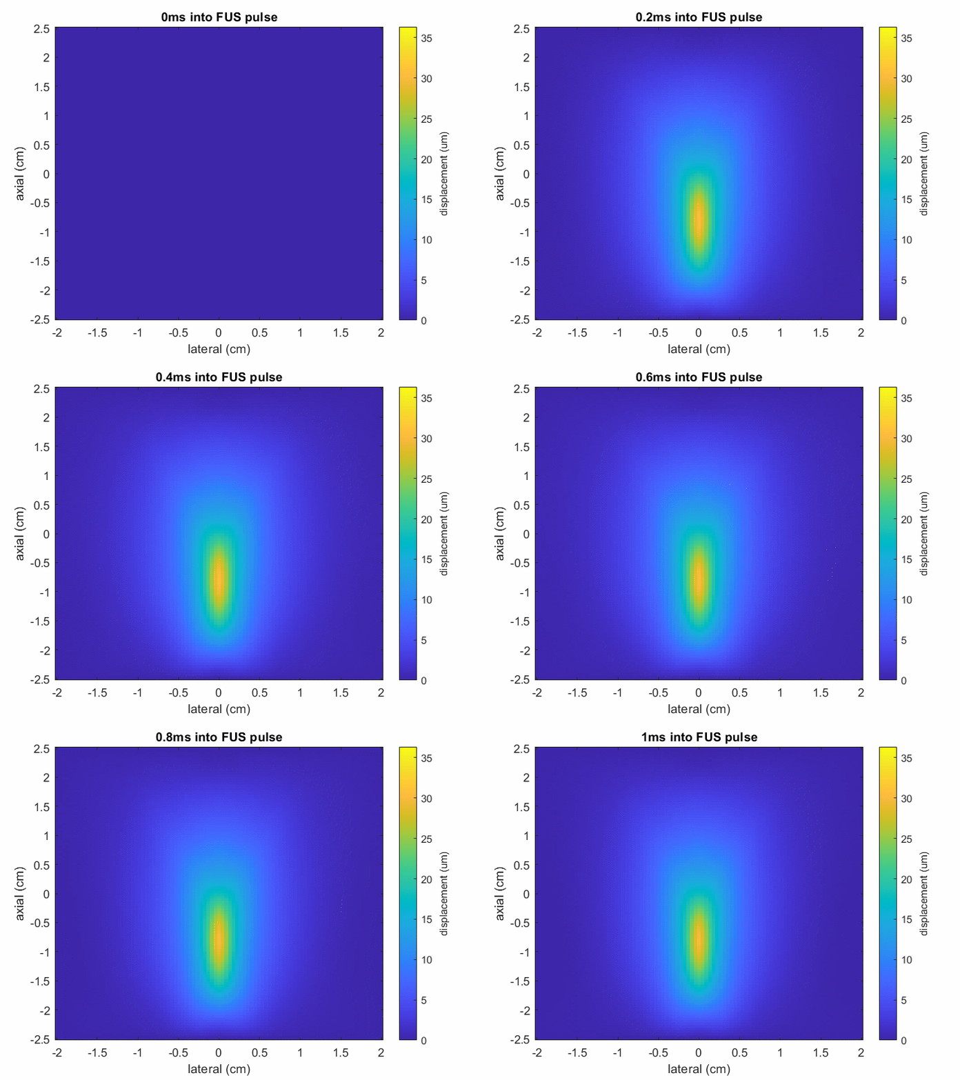
SimulationsAn 850kHz single element ultrasound transducer with a 64mm diameter and 63.2mm focus was simulated in k-Wave3 (Figure 2) across a range of pressure levels from 0.27 to 2.70MPa. The average acoustic intensity (I) was calculated from each simulated pressure field and converted to acoustic radiation force using F = 2a I / c where I is average pressure-squared, alpha is the tissue attenuation coefficient, and c is the speed of sound. The force maps were input to a finite element method (FEM) solver to calculate displacements during MR-ARFI pulses up to 4 ms in duration (Figure 3). FEM-based calculations were performed over a radially symmetric 2.0x2.0x2.5 cm3 slice around the focus with (100,100,150) nodes. The transducer was switched ‘on’ for 4ms of the 5ms FEM calculation, corresponding to a motion encoding gradient (MEG) duration up to 4ms. A Poisson’s ratio of 0.49, and a Young’s modulus of 2000Pa were used, the timestep was 5x10⁻⁵s. The resulting dynamic displacement maps were used to calculate the expected phase maps for a given motion encoding gradient (MEG) duration, which were then converted back to average displacement during the MEG.
Phantom Experiments
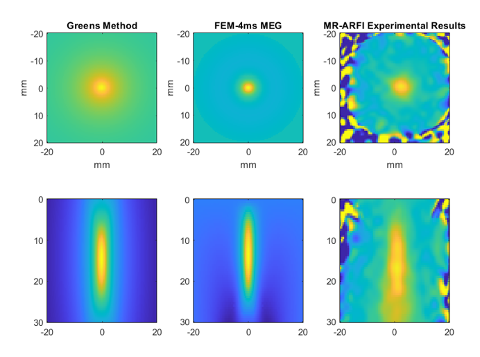
The focal displacement FWHM’s of MR-ARFI maps generated by a Green’s theorem PSF-based steady state displacement calculation method4 and the FEM-simulated ARFI maps were compared to phantom experiments with the transducer described above (Figure 4). Phantom experiments were performed in a 3T Philips Elition MR scanner with an agar-graphite phantom5. Because the stiffness of the phantom was unknown, all simulated displacements were normalized to the maximum observed displacement in the phantom, 2.5µm.
Lookup table
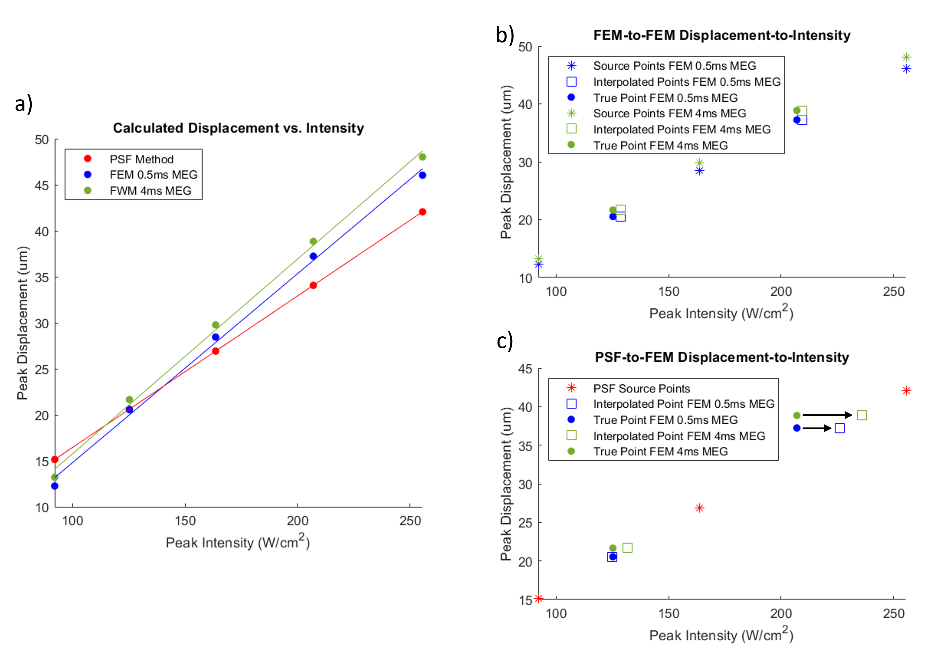
Acoustic pressure fields were simulated across a range of intensities and input to the PSF and FEM methods to calculate MR-ARFI displacements. The minimum, middle, and maximum displacements and corresponding intensities were used as source points in lookup table calculations to interpolate the ‘unknown’ intensities of the middle points, given their displacement. The predicted intensities were compared between PSF- and FEM-based MR-ARFI maps.
Results
The FWHM of the coronal slices were 10mm for the PSF method, 2.7mm for FEM and 6.4mm for phantom measurements. The axial FWHM were 30.75mm for the PSF method, 23mm for FEM and 18.7mm for phantom measurements.While displacement and intensity varied perfectly linearly with the PSF method, it did not for the FEM method, for either MEG duration. Lookup tables were created to calculate the intensity for a given displacement for the PSF, and FEM methods. Error was less than 3W/cm2 when using FEM source points to interpolate pressure from FEM displacement. When using the PSF method as a source and FEM displacement to calculate the intensity, the error between interpolated intensity and known intensity was 19.25W/cm2, 9% of the true intensity, for FEM with a 0.5ms MEG, and 29.07W/cm2, 14% of the true intensity for FEM with a 4ms MEG.
Discussion & Conclusion
We have reported a comprehensive model of MR-ARFI displacement map generation which relates acoustic intensity or pressure to displacement, and accounts for time-varying displacement over the duration of a motion encoding gradient/FUS pulse pair. The method was used in an initial study to invert displacement measurements to obtain acoustic intensity. This will enable the further development of inverse methods for MR-ARFI-based acoustic dosimetry in FUS neuromodulation.Acknowledgements
Grant Support : 3T32EB007509-17S1, UG3 NS 135551References
[1] N. McDannold and S. E. Maier, “Magnetic resonance acoustic radiation force imaging,” Medical Physics, vol. 35, no. 8, pp. 3748–3758, 2008.
[2] M. A. Phipps, S. V. Jonathan, P.-F. Yang, V. L. Chaplin, L. M. Chen, W. A. Grissom, and C. F. Caskey. Considerations for ultrasound exposure during transcranial MR acoustic radiation force imaging. Sci Rep, 9:16235, 2019.
[3] B. E. Treeby and B. T. Cox, "k-Wave: MATLAB toolbox for the simulation and reconstruction of photoacoustic wave-fields," J. Biomed. Opt., vol. 15, no. 2, p. 021314, 2010.
[4] A. Payne, J. De Bever, A. Farrer, B. Coats, D. L. Parker, and D. A. Christensen, “A simulation technique for 3D MR-guided acoustic radiation force imaging,” Medical Physics, vol. 42, no. 2, pp. 674–684, Feb. 2015.
[5] H. Luo et al., “Reduced-field of view three-dimensional MR acoustic radiation force imaging with a low-rank reconstruction for targeting transcranial focused ultrasound,” Magnetic Resonance in Medicine, vol. 88, no. 6, pp. 2419–2431, 2022.
[6] P.-F. Yang et al., “Differential dose responses of transcranial focused ultrasound at brain regions indicate causal interactions,” Brain Stimulation, vol. 15, no. 6, pp. 1552–1564, Nov. 2022.
Figures