Introduction

Quantitative Magnetic Resonance Imaging (qMRI) has gained a lot of attention recently. To develop, test and benchmark MRI methodology to accurately measure quantitative MRI parameters, phantoms containing materials with ranges of the parameters of interest are often used.¹ However, most MRI parameters, such as T1, T2, proton density, and the diffusion coefficient, have temperature dependences.² To accurately evaluate new methods of measuring these parameters, the absolute temperature within the phantom must be accurately known. Ideally this temperature would be measured using MRI, rather than external probes, but most MR thermometry approaches only measure relative temperature change. It is, however, possible to measure absolute temperatures with MRI using spectroscopic (imaging) approaches, where protons in a temperature insensitive environment are used as reference to protons in a temperature sensitive environment.
In this work we demonstrate the use of an MR spectroscopic imaging approach to rapidly, accurately and precisely measure temperature at multiple locations throughout a qMRI phantom. The temperature dependent spacing between the two hydrogen peaks (CH2 and OH) of ethylene glycol (EG) (C₂H₆O₂) was calibrated and used to compute absolute temperature.³ A reconstruction pipeline to automatically calculate the temperatures is presented and experiments are performed over a wide temperature range (~7 – 37 °C) on multiple scanners.

Methods

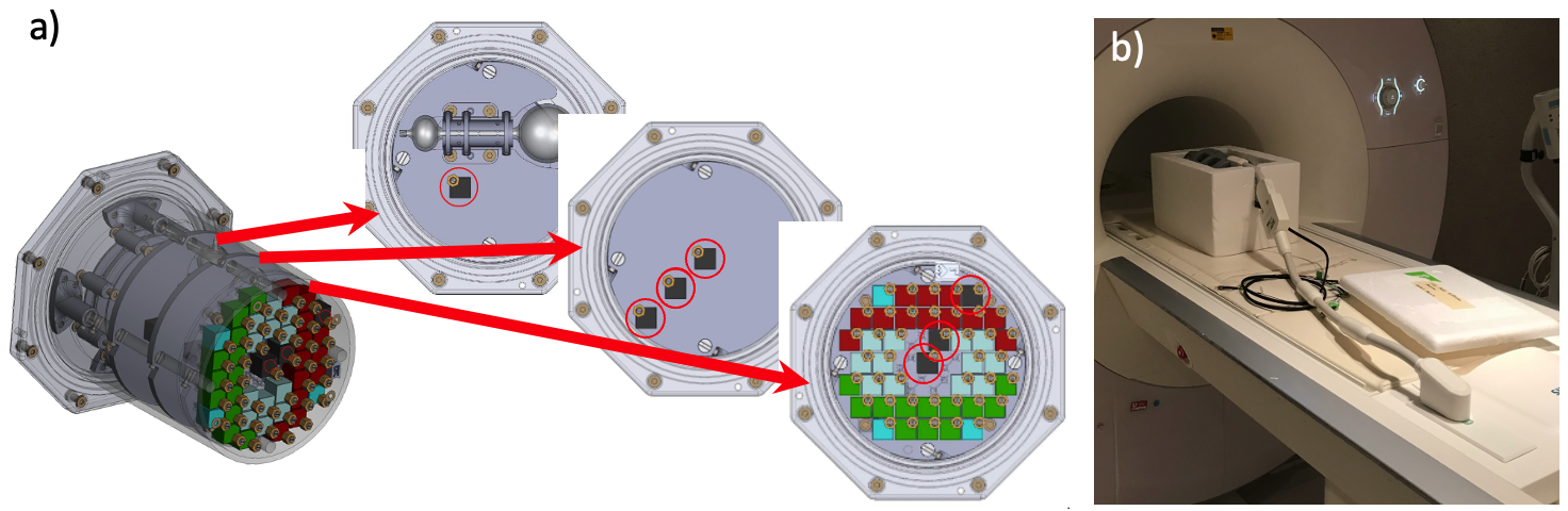
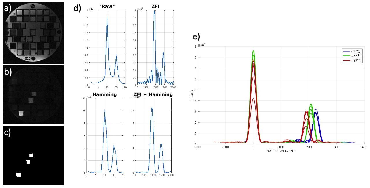
A qMRI phantom (Psychology Software Tools, Pittsburgh, PA, USA), 16 x 28 cm (diameter x length), was fitted with seven EG cubes (~1.5 cm³) spread over three slices, Figure 1. Fiber optic probes (Osensa Innovations, Burnaby, BC, Canada) were placed in 5 vials and used for calibration. The temperature of the vials was measured immediately before and after all scans. Experiments were performed on two different 3T MRI scanners (Prisma and Vida, Siemens Healthineers, Erlangen, Germany) to test reproducibility between scanners. On both scanners OEM spine and flex coils were used for signal detection. The pulse sequence was a modified spoiled gradient recalled echo sequence, adjusted to acquire 32 echoes with the following parameters: monopolar readout, FOV=192x192 mm, 1x1 mm voxel size, 3 slices covering the three planes with EG cubes, 2 mm slice thickness, TR=234 ms, TE=3.0-74.9 ms in steps of 2.3 ms, acquisition time 45 sec. The phantom was scanned at three different temperatures; cold ~7 °C, room temperature ~22 °C, and warm ~37 °C, after equilibrating at each temperature for at least 24 h. At each temperature, three repeated scans were performed on different days, for a total of 9 scans per scanner.
All image reconstruction and data processing were performed using Matlab (Natick, MA, USA). A simple reconstruction pipeline was used to automatically locate the EG cubes. After image reconstruction a magnitude-based threshold was applied to the average difference between sequential echoes. The resulting image was further processed with a dilate operation to fill any holes followed by an erode operation to prevent the inclusion of EG bordering voxels, Figure 2. Once the EG cubes were spatially located an FFT in the echo dimension was performed to find the spectrum. A Hamming filter was applied to reduce Gibb’s ringing and zero fill interpolation was performed to reduce partial volume effects, Figure 2. In the resulting spectra, a single large peak (CH2) and a second smaller peak (OH) could easily and automatically be detected, Figure 2. The mean and variance of the peak spacing within each EG vial was computed and used together with the fiber optic probe measurements to “calibrate” the peak spacing to absolute temperature. The regression analysis was performed using all data (18 scans x 5 vials with probes for both scanner) as well as scanner-by-scanner and temperature-range-by-temperature-range.

Results

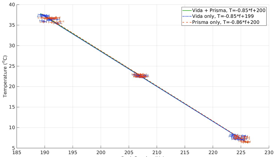
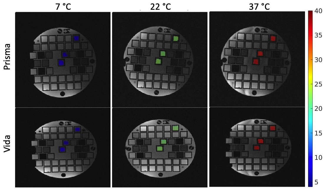
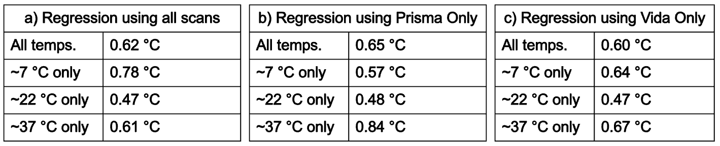
Figure 3 shows linear regression to all 18 scans, as well as individually by scanner, with fitted values for the three cases listed in the legend. Example of temperature maps are shown in Figure 4. Table 1 summarizes root-mean-square-error for regression to all data (a) and individually per scanner (b) and c)). In each case, RMSE is calculated collectively for the three temperatures, and also individually by temperature.

Discussion and Conclusions

A ME-GRE approach for spectroscopic imaging is presented and shown to give rapid (~15 s/slice) and precise (0.5 – 1.0 °C) temperature measurements in multiple planes throughout a qMRI phantom. The measurements were most accurate around 22 °C (SD<0.5°C), which is where the fiberoptic probes were calibrated, with slightly lower accuracy around 7 and 37 °C (SD~0.6-0.8°C). These observations were true both when evaluating the data from both scanners together, and each scanner individually. This observation makes the approach promising to be widely generalized, but cross-vendor and field strength evaluation is needed.

Acknowledgements

NIH grants R01EB028316, S10OD026788 and S10OD018482, and Department of Veterans Affairs I01RX003444.