2704

Recurrent reconstruction network enables real-time and high-resolution PRF thermometry for LITT

Yuancheng Jiang¹, Ziyi Pan¹, Kai Zhang², Meng Han³, Wenbo Liu³, Guangzhi Wang⁴, and Hua Guo¹
¹Center for Biomedical Imaging Research, Department of Biomedical Engineering, School of Medicine, Tsinghua University, Beijing, China, ²Beijing Tiantan Hospital, Capital Medical University, Beijing, China, ³Sinovation Medical, Beijing, China, ⁴Department of Biomedical Engineering, School of Medicine, Tsinghua University, Beijing, China

Synopsis

Keywords: Thermometry/Thermotherapy, Thermometry

Motivation: Proton-resonance-frequency (PRF) shift-based thermometry is used to monitor the temperature change during Laser-interstitial-thermal-therapy (LITT). Recent LITT developments call for PRF thermometry to achieve larger volume coverage and higher spatiotemporal resolution for enhanced therapeutic efficacy.

Goal(s): Accelerate the PRF thermometry by compressed-sensing (CS) undersampling to enlarge the volume coverage and increase the spatiotemporal resolution. Use a neural network for real-time reconstruction of the undersampled data.

Approach: A recurrent reconstruction network (RRN) was proposed to reconstruct the highly undersampled PRF data. Retrospective and prospective undersampling experiments were conducted.

Results: RRN demonstrated good image reconstruction quality in retrospective experiments, with promising results in prospective experiments.

Impact: The introduction of the RRN offers a solution for real-time and high-resolution PRF thermometry during LITT, potentially improving treatment outcomes.

Introduction

LITT is a minimally invasive clinical method that employs laser-induced heating to ablate pathological tissues.¹ During LITT, PRF thermometry is widely used to monitor the temperature change of the heating zone.² Recent LITT practices require PRF thermometry to achieve larger volume coverage and higher spatiotemporal resolution to enhance therapeutic efficacy. To meet this requirement, CS-undersampling³ is often used to accelerate the data sampling. But the reconstruction time of CS-undersampled data is usually long and cannot meet the clinical demand for real-time temperature monitoring. In this work, a recurrent-reconstruction-network (RNN) is hence introduced for real-time reconstruction of the CS-undersampled PRF data. Retrospective and prospective undersampling experiments were conducted for evaluation.

Methods

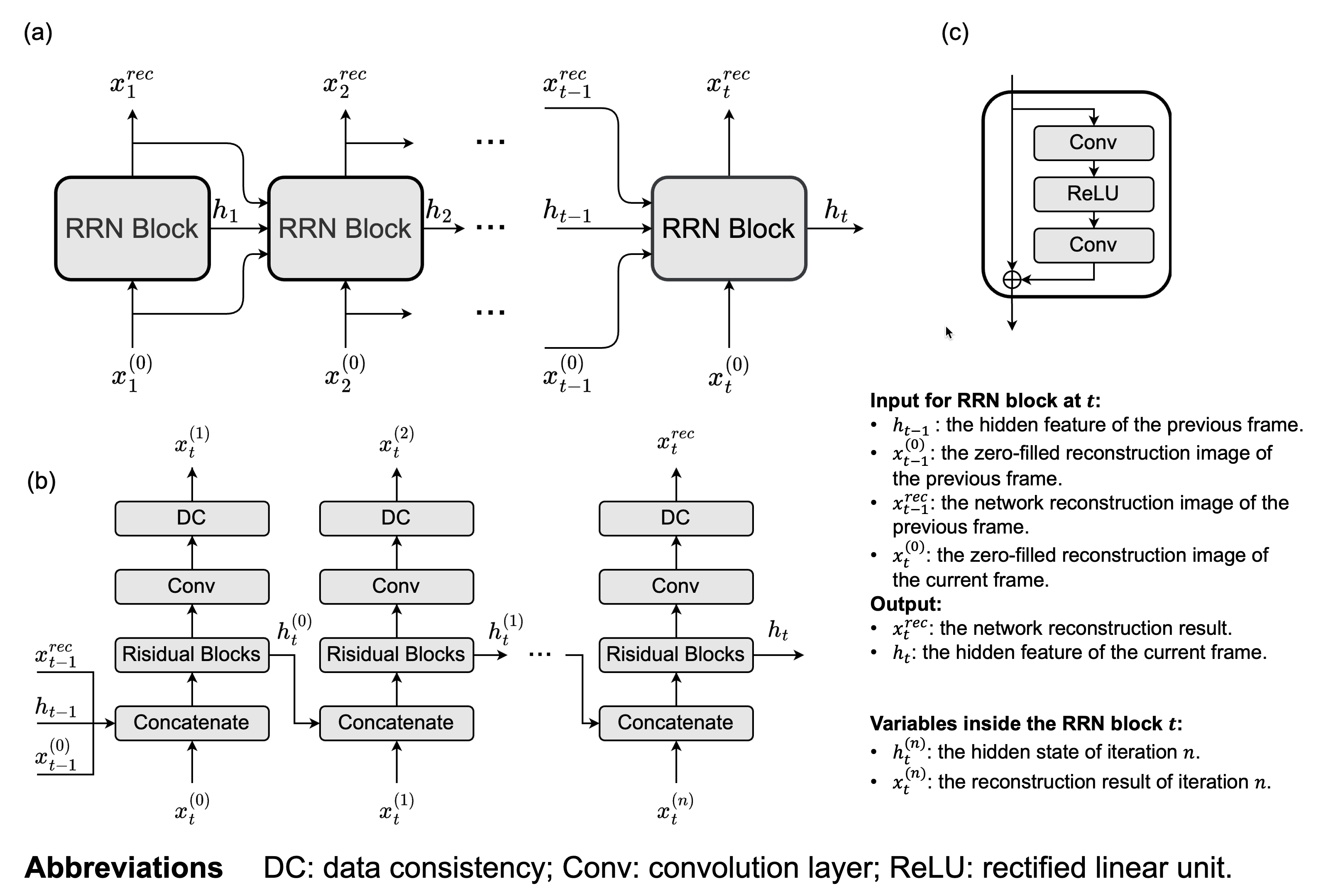
Network architecture
The network structure is shown in Fig 1(a). Each RRN block takes data from the current and the previous frames as input, utilizing temporal redundancy in PRF data for robust reconstruction. The structure inside each RRN block is shown in Fig 1(b) and Fig 1(c).

Data acquisition
PRF data were collected during the LITT treatments for 18 epilepsy patients in Beijing Tiantan Hospital, on a Siemens Verio 3T scanner. The studies received local IRB approval. The heating procedure was conducted by a clinical laser applicator (MRI-Guided Laser Ablation System, Sinovation Medical, Beijing, China). Data from each patient is an image series with multiple frames. We selected the series from 14 patients as the training set, 1 as the validation set, and 3 as the test set.

Network Training and temperature calculation
The acquired fully-sampled image series and the undersampled series, which were 8-fold CS-undersampled⁴ in k-space, were taken as training pairs. Before network input, the magnitude images of all series were normalized to [0,1] and the real and imaginary parts of images were split to two different network-input channels. For a given series, the temperature change of each frame was acquired by calculating the phase difference map between that frame and the reference frame (averaged first five frames).

Retrospective experiment
A retrospective undersampling experiment was performed. Images from the test set were retrospectively CS-undersampled and reconstructed by RRN. Three conventional CS-reconstruction methods (dTV⁵, L+S⁶, AscLR⁷), and another deep-learning method (CRNN^8,9) were used for comparison. The magnitude SSIM between the reconstruction results and the original images was calculated to evaluate the magnitude reconstruction performance. Temperature results were evaluated by pixel-wise temperature RMSE (tRMSE). Due to the ‘lazy start’ issue of the recurrent network, the first 15 frames (~60 s) were excluded when calculating the quantitative metrics.

Prospective experiment
We also conducted a prospective undersampling experiment for further evaluation. A gel phantom was scanned on a Philips Ingenia CX 3T scanner using an 8-fold CS undersampled 2D GRE sequence to get the high-resolution PRF data (12 slices). During scanning, the phantom was heated using the previously mentioned laser applicator for about 3 minutes, followed by cooling. A temperature measurement optical sensor (LUXTRON M920, Advanced Energy, USA) was placed near the heating center to monitor the temperature. RRN was used to reconstruct the undersampled data and the temperature results were compared to the temperature captured by the optic sensor.

Results and discussion

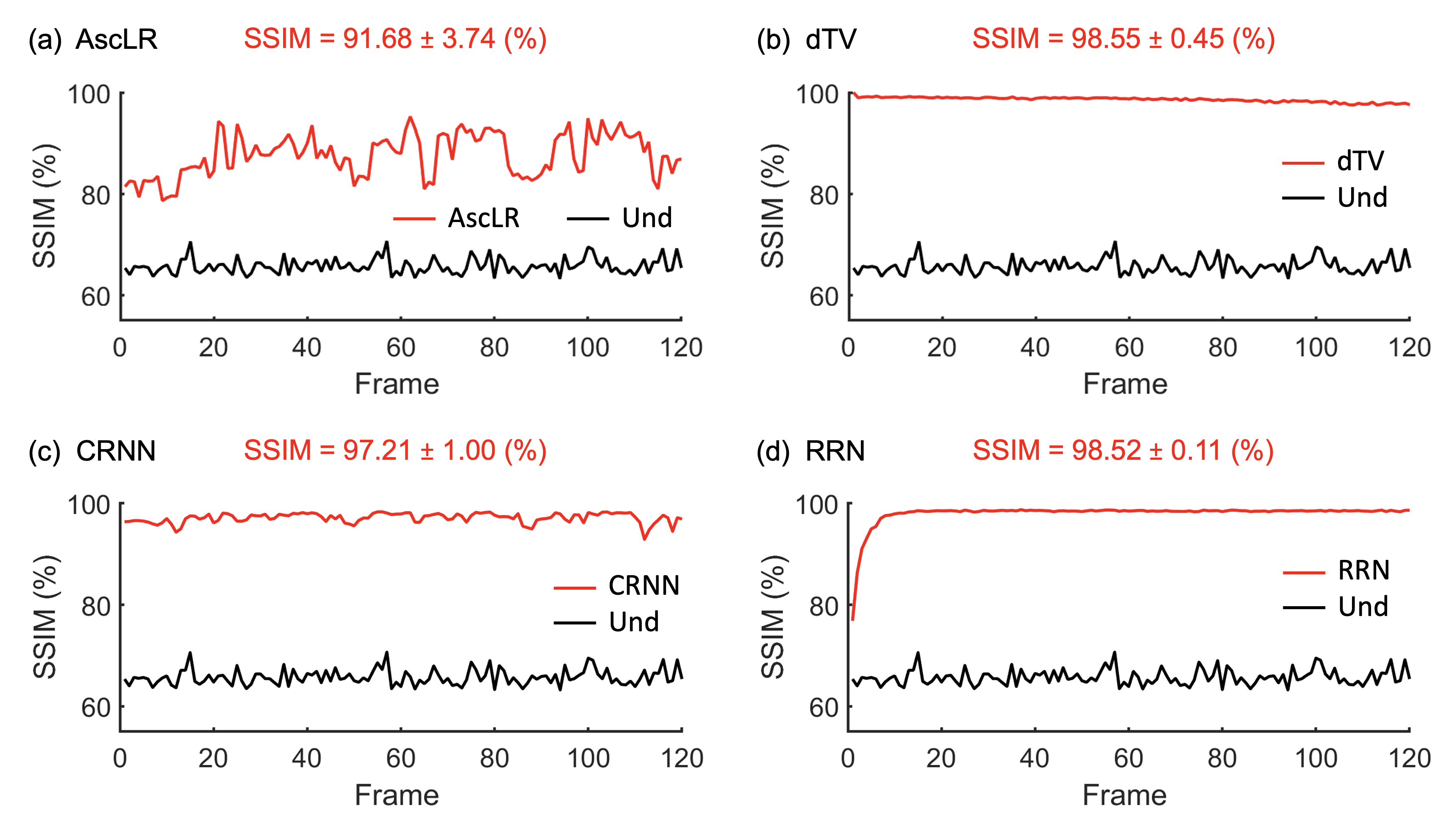
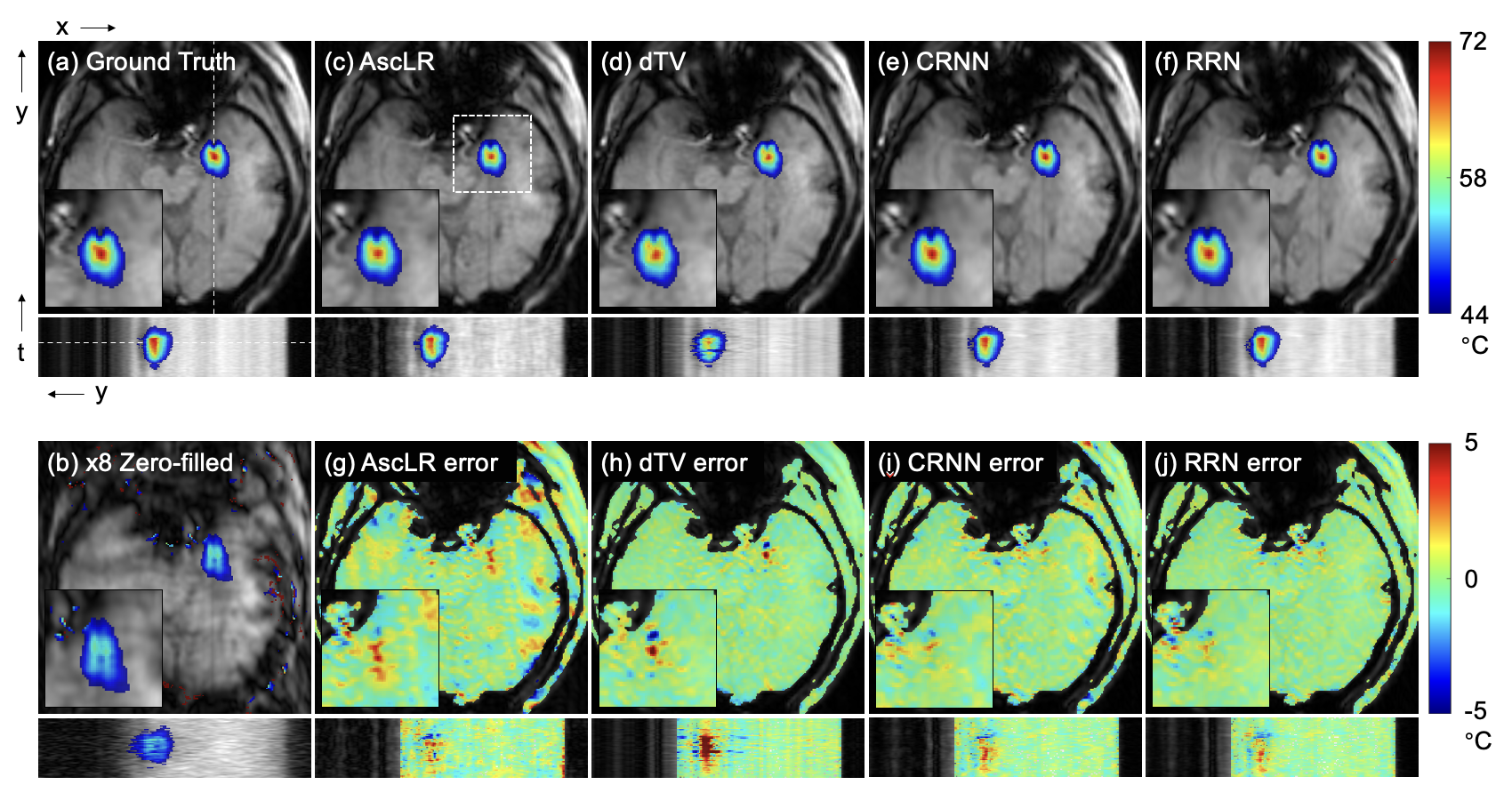
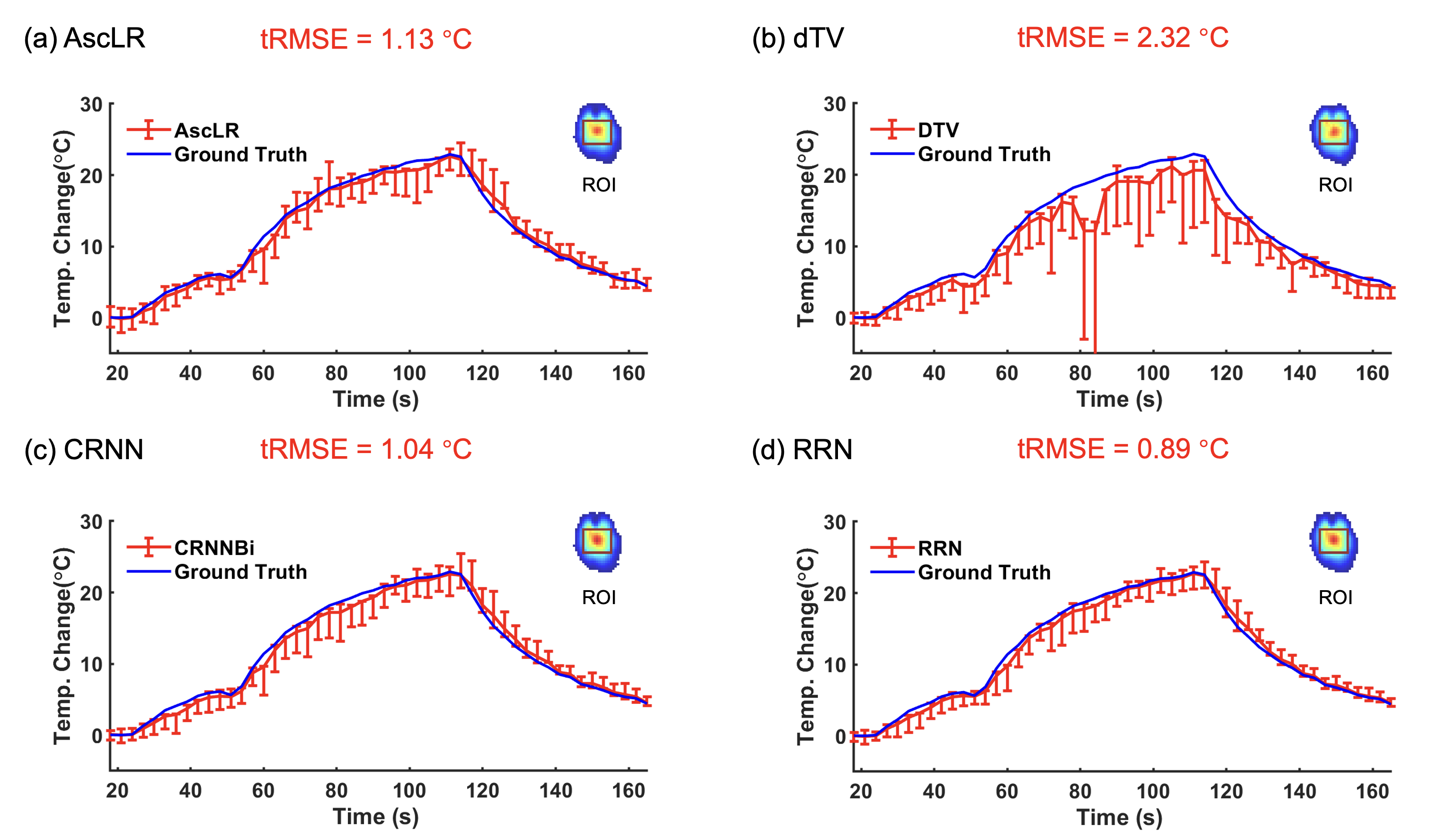
Retrospective experiment
The RRN achieves an average frame reconstruction time of 9 ms, demonstrating its real-time reconstruction capability. Fig 2 presents the magnitude SSIM curve for each method. RRN and dTV have the overall best SSIM, despite the initial frames of RRN having the ‘lazy start’ issue. In Fig 3, RRN and CRNN demonstrate the best temperature reconstruction ability. The temperature curve is shown in Fig.4, where RRN shows the smallest error and the lowest tRMSE.

Prospective experiment
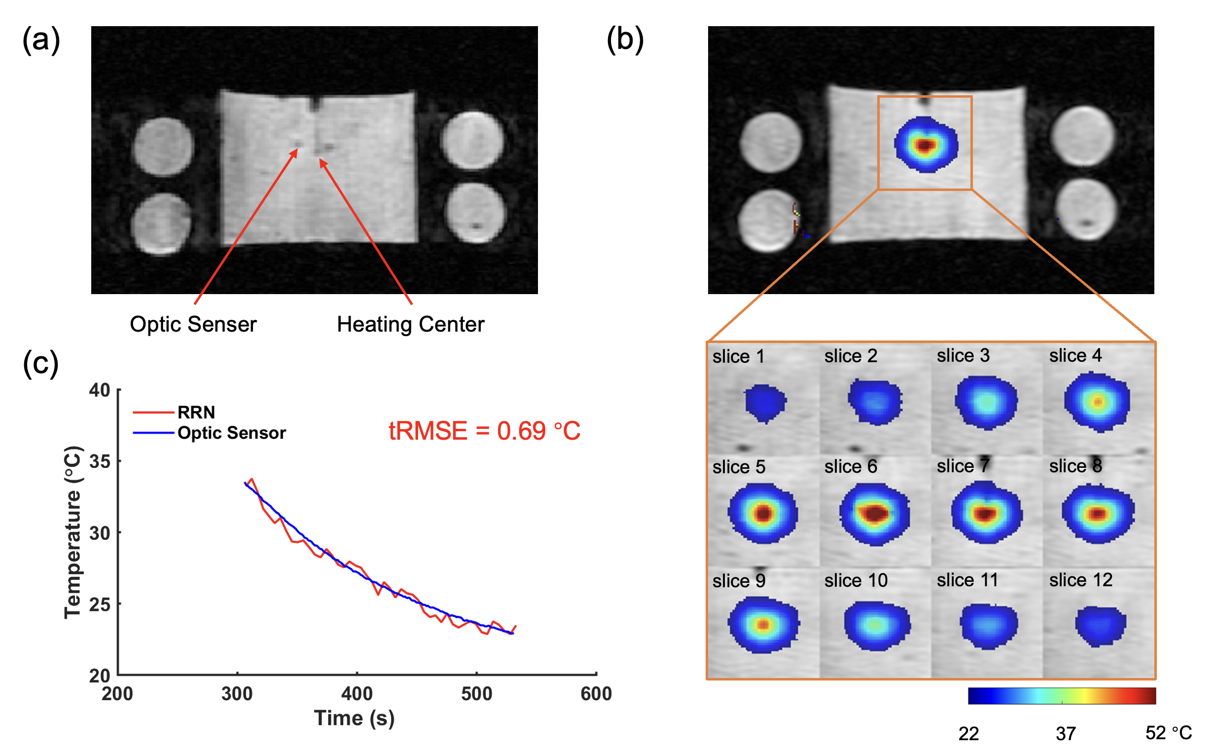
In Fig 5(a), the RNN reconstructed magnitude result of the prospective undersampled data is displayed, with the location of the optic sensor and heating center visible. Fig 5(b) shows the well-reconstructed temperature maps for all 12 slices at 261 s. Fig 5(c) presents the temperature curve of RRN, closely matching the optic sensor curve with low tRMSE (only the cooling down phase is shown because the optic sensor cannot monitor the temperature during heating).

There are still some artifacts in the RRN reconstruction result, which is probably because it was trained on human data, without fine-tuning on phantom data. But it still shows promise. Our next steps involve establishing a reliable pipeline for real-time data transmission, reconstruction, and visualization. We will also conduct a more in-depth investigation into RRN.

Conclusion

Retrospective and prospective experiments demonstrate the ability of our RRN method to reconstruct the highly CS-undersampled PRF data, indicating the possibility of using CS-undersampling and RRN reconstruction for high-resolution and large volume coverage PRF thermometry.

Acknowledgements

No acknowledgement found.

References

1. Salem U, Kumar VA, Madewell JE, et al. Neurosurgical applications of MRI guided laser interstitial thermal therapy (LITT). Cancer Imaging 2019;19(1).

2. Blackwell J, Krasny MJ, O'Brien A, et al. Proton Resonance Frequency Shift Thermometry: A Review of Modern Clinical Practices. J Magn Reson Imaging 2020.

3. Lustig M, Donoho D, Pauly JM. Sparse MRI: The application of compressed sensing for rapid MR imaging. Magnetic Resonance in Medicine 2007;58(6):1182-1195.

4. Schlemper J, Caballero J, Hajnal JV, Price AN, Rueckert D. A Deep Cascade of Convolutional Neural Networks for Dynamic MR Image Reconstruction. IEEE Transactions on Medical Imaging 2018;37(2):491-503.

5. Chen C, Li Y, Axel L, Huang J. Real time dynamic MRI by exploiting spatial and temporal sparsity. Magnetic Resonance Imaging 2016;34(4):473-482.

6. Otazo R, Candès E, Sodickson DK. Low-rank plus sparse matrix decomposition for accelerated dynamic MRI with separation of background and dynamic components. Magnetic Resonance in Medicine 2015;73(3):1125-1136.

7. Wang F, Dong Z, Chen S, et al. Fast temperature estimation from undersampled k-space with fully-sampled center for MR guided microwave ablation. Magnetic Resonance Imaging 2016;34(8):1171-1180.

8. Qin C, Schlemper J, Caballero J, Price AN, Hajnal JV, Rueckert D. Convolutional Recurrent Neural Networks for Dynamic MR Image Reconstruction. IEEE Transactions on Medical Imaging 2019;38(1):280-290.

9. Pan Z, Zhang J, Zhang K, et al. Real-time Reconstruction for Accelerated MR Thermometry Using CRNN in MRgLITT Treatment. Proc ISMRM. 2022. 3187.

Figures

Fig 1 RRN structure. (a) The overall structure of RRN. (b) The structure inside each RRN block. 4 input tensors are concatenated along the channel dimension and then pass through multiple residual blocks. The output $$$h_t^{(0)}$$$then undergoes a Conv and DC layer to yield the result for the first iteration $$$x_t^{(1)}$$$. Both of them go to the next iteration thereafter. After n iterations, the final result and hidden feature for the next frame are produced. (c) The residual block in (b). It is two Conv layers with a ReLU, and with the outer layer connected by skip connections.

Fig 2 SSIM curves from reconstructed magnitude results of one 8× undersampled data (Retrospective exp.). The ground truth data were acquired by a spoiled GRE sequence. Parameters: flip angle = 30°, TE/TR = 11.6/76 ms, matrix = 128×128, resolution = 1.8×1.8 mm², slice thickness = 5 mm, slice number = 3, GRAPPA = 3, temporal resolution = 3 s/frame. In each subplot, the red curve is the SSIM between the reconstructed result and the ground truth. The black curve is from the zero-filled result. On the top of each subplot, the overall SSIM metric over the temporal dimension is annotated as mean ± std.

Fig 3 Magnitude (background) and temperature (in colormap) results of one 8× undersampled data (Retrospective exp.). Each subfigure has x-y and y-t images. The dashed line in subfigure (a) on the x-y image represents the location where the y-t image is intercepted, and vice versa. In each x-y image, the bottom-left corner is an enlarged view of the heating ROI, which is outlined by a dashed box in subfigure (c). (a)-(f) Magnitude and temperature results of different methods. (g)-(j) Temperature errors of the results from each method with respect to ground truth.

Fig 4 Temperature curves within the ROI for one 8× undersampled data (Retrospective exp.). 50 frames are shown. The ROI area around the heating center is outlined by a rectangular within the temperature colormap in the top right corner of each subplot. On the top of each subplot is the tRMSE. In each subplot, the blue curve is the average temperature of the ground truth within the ROI, while the red curve is the average temperature from each reconstruction method. The red error bars indicate the minimum and maximum error within the ROI, at each time point.

Fig 5 The prospective experiment results. The data is acquired by a specifically designed GRE sequence. Parameters: flip angle = 16°, TE/TR = 13/20 ms, matrix = 128×128, resolution = 1.8×1.8 mm², slice thickness = 1.8 mm, CS undersample rate = 8, temporal resolution = 4.8s/frame. (a) The magnitude result of slice 7. The location of the heating center and optic sensor is pointed. (b) The temperature results from each slice of a frame. (c) The temperature curves measured by the optic sensor and reconstructed by RRN. The top-right corner is the calculated tRMSE between two measurements.

Proc. Intl. Soc. Mag. Reson. Med. 32 (2024)

2704

DOI: https://doi.org/10.58530/2024/2704