2612
Robust and Repeatable Quantitative Susceptibility Mapping for Head and Neck Squamous Cell Carcinoma1Department of Medical Physics and Biomedical Engineering, University College London, London, United Kingdom, 2UCL Cancer Institute, University College London, London, United Kingdom, 3Guy's and St Thomas' NHS Foundation Trust, London, United Kingdom
Synopsis
Keywords: Susceptibility/QSM, Head & Neck/ENT
Motivation: Identifying hypoxia in head and neck squamous cell carcinoma (HNSCC) could improve treatment. Quantitative susceptibility mapping (QSM) offers a potential method for measuring tissue composition and oxygenation.
Goal(s): To develop a robust, repeatable pipeline for QSM in the head and neck region.
Approach: We tested various QSM reconstruction pipelines and compared their intra- and inter-session repeatability, before applying an optimized pipeline to a HNSCC patient dataset.
Results: A pipeline using ROMEO phase unwrapping, V-SHARP background field removal, and iterative Tikhonov susceptibility calculation was found to be more repeatable than the previously reported best pipeline and showed nodal susceptibility differences in a HNSCC patient.
Impact: This new optimized pipeline provides repeatable susceptibility values in key ROIs through the head and neck region and detected nodal susceptibility differences in a HNSCC patient. Therefore, it is applicable for clinical studies of tissue susceptibility and oxygenation in HNSCC.
Introduction
Hypoxia has been shown to be an indicator of lower survival and poor treatment response in Head and Neck Squamous Cell Carcinoma (HNSCC).1,2 Recent work has shown that Quantitative Susceptibility Mapping (QSM)3,4 can be used to measure oxygenation in the brain,5,6 and this can be extended to other parts of the body.7,8 The head and neck (HN) region presents unique challenges for QSM, including fat-water phase artifacts, flow effects, physiological motion, and the presence of multiple air-tissue interfaces. For tissue susceptibility values ($$$\chi$$$) provided by QSM to be clinically useful, the acquisition and reconstruction process must be repeatable. Previous work has been undertaken to develop an optimized HN QSM pipeline,9 and here we demonstrate the repeatability of a further improved QSM pipeline in healthy volunteers, and show its applicability in HNSCC patients.Methods
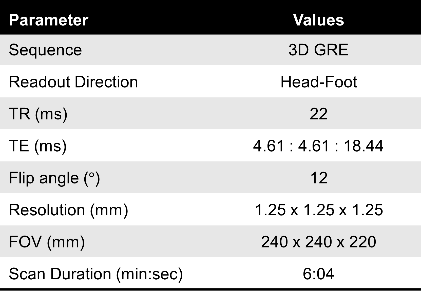
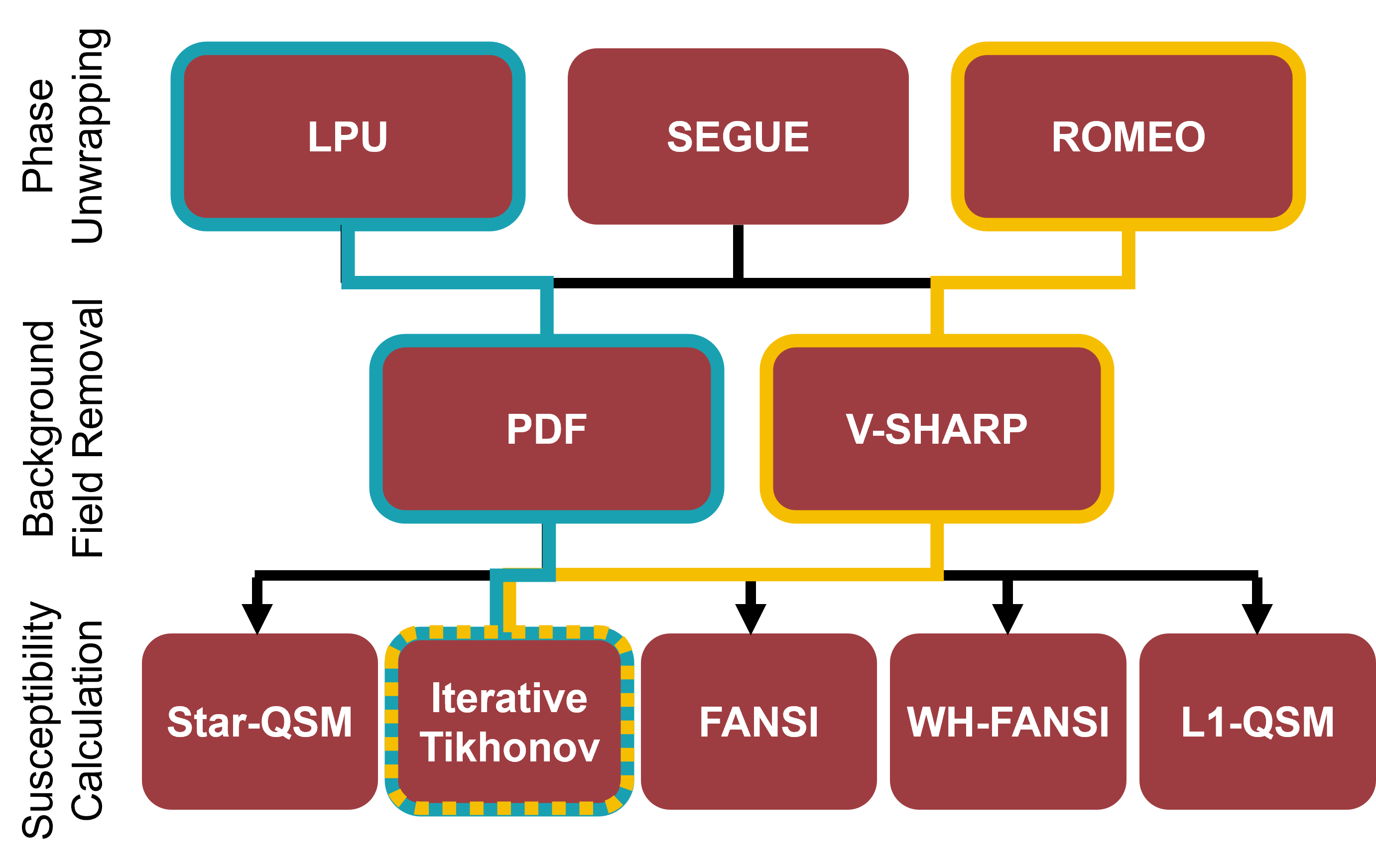
Multi-echo HN QSM images from 10 healthy volunteers (acquired for previous study9) were used to test a range of QSM reconstruction pipelines and quantify the repeatability of the optimized pipeline. Each subject was scanned three times per session, for two sessions one week apart. Data were acquired on a 3T Achieva system (Philips, Netherlands) using a 3D-GRE sequence (sequence parameters shown in Figure 1). HN QSM images from one HNSCC patient (Male, 58, T4N2bM0 larynx) were acquired on a 3T Skyra system (Siemens, Germany).Multi-echo images were combined using non-linear field fitting,10 and, in the remaining stages of the QSM reconstruction pipeline, multiple methods were tested based on recent literature, as shown in Figure 2. Phase unwrapping methods tested were: Laplacian phase unwrapping (LPU11), a region-growing method (SEGUE12), and a path-based method (ROMEO13). Background field removal methods tested were: Projection onto dipole fields (PDF)14 and V-SHARP.15 Susceptibility calculation methods tested were: iterative Tikhonov-regularized inversion (iTik),9 FANSI,16 Star-QSM,17 Weak-harmonic regularized FANSI,16,18 and L1-QSM.19 Processing and analysis were conducted in MATLAB (MathWorks, Natick, MA).
Regions of interest (ROIs) in the brain and HN were obtained by a combination of automatic segmentation using FSL FIRST20 and manual segmentation checked by an experienced radiologist. Average $$$\chi$$$ values in each ROI were used to calculate both intra- and inter-session repeatability coefficients $$$RC$$$.21
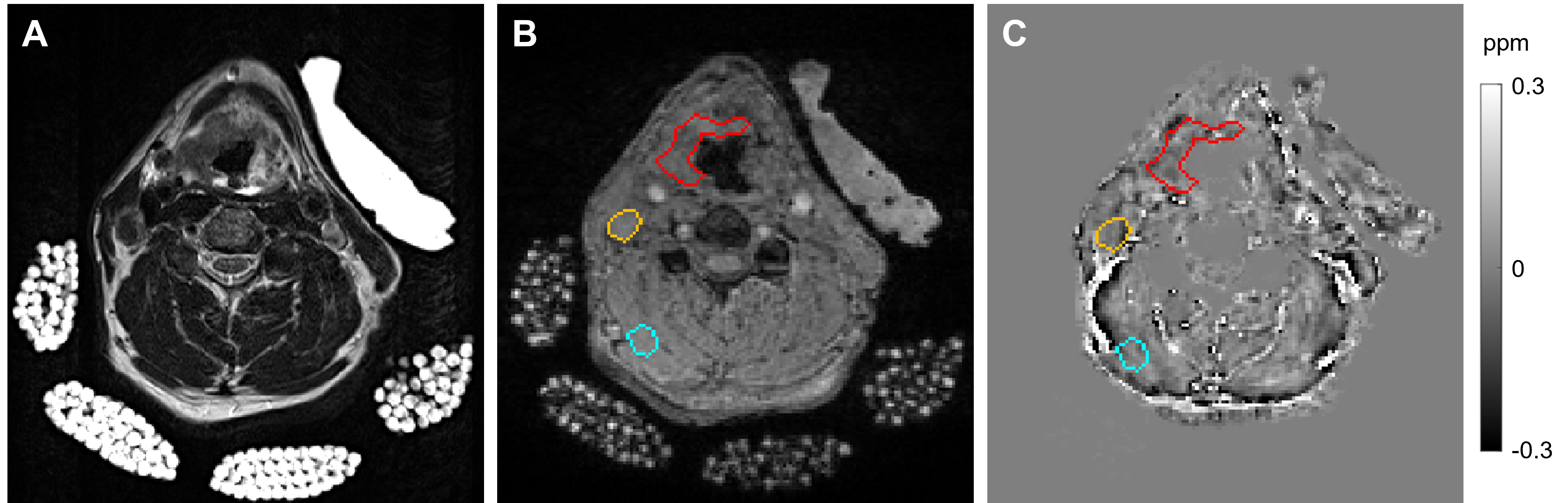
The optimized pipeline was applied to reconstruct a QSM from the HNSCC patient, and $$$\chi$$$ values were extracted from manually drawn ROIs (primary tumour, lymph node, sternocleidomastoid muscle). These were compared for significant differences with ANOVA.
Results
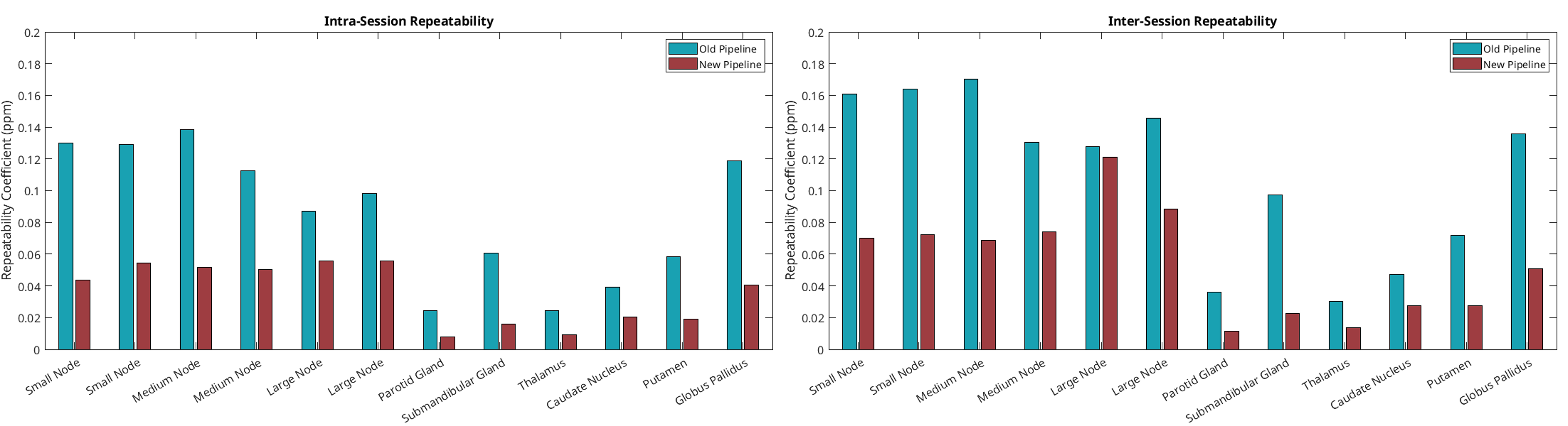
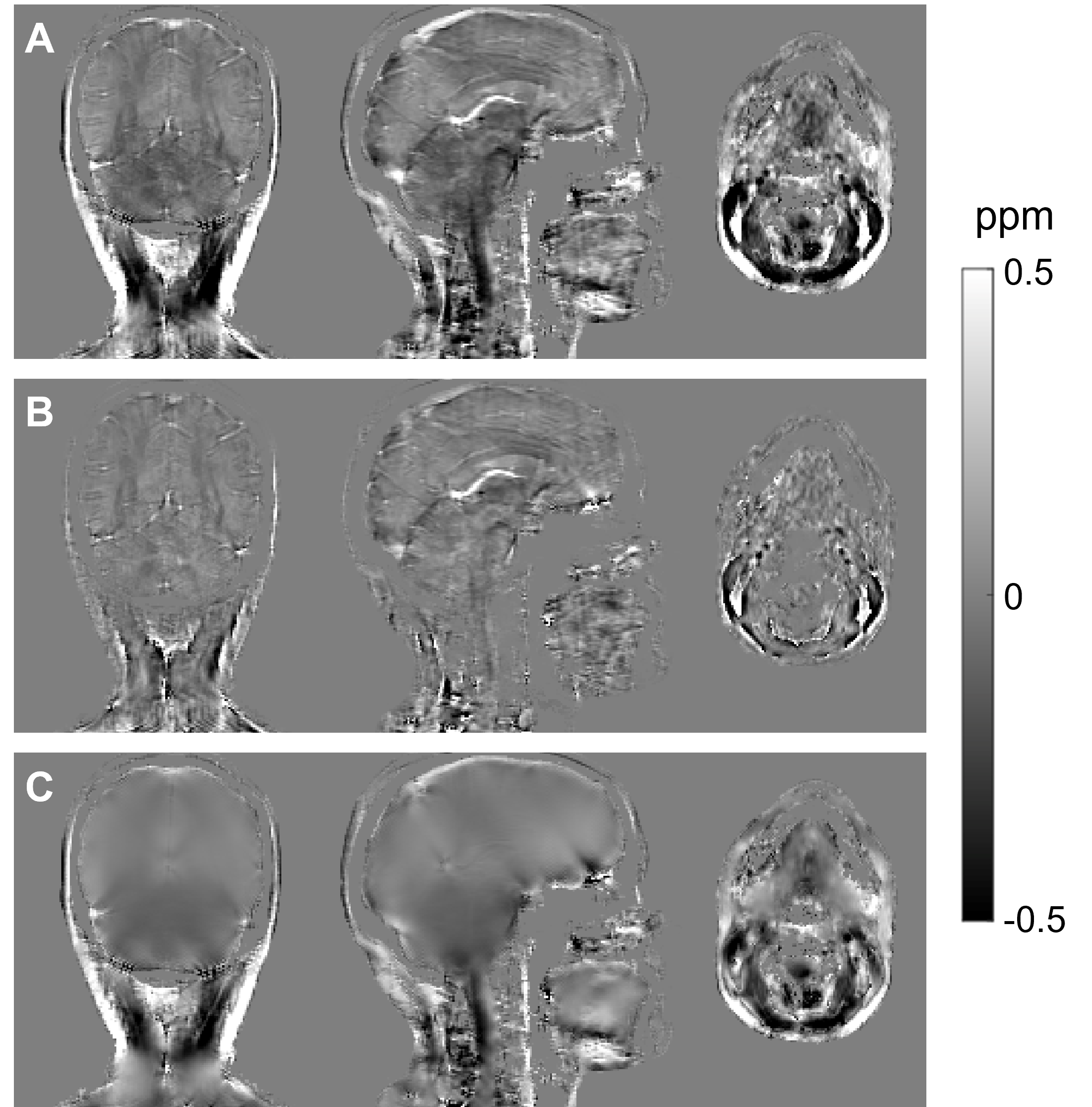
Visual assessments and distributions of susceptibility values in HN ROIs were used as an initial comparison between different techniques for the three stages of QSM reconstruction. A ‘new’ optimized pipeline consisting of ROMEO13 phase unwrapping, V-SHARP15 background field removal (an optimal V-SHARP kernel size (22 mm) was found by maximizing contrast between susceptibility values in brain ROIs), and iTik9 susceptibility calculation, was compared with the ‘old’ pipeline for intra-session and inter-session repeatability (Figure 3). $$$RC_{intra-session}$$$ was 0.085ppm for the old pipeline and 0.035ppm for the new optimized pipeline. $$$RC_{inter-session}$$$ was 0.11ppm for the old pipeline and 0.054ppm for the new pipeline. Figure 4 shows the differences between the two pipelines in a representative subject.In the HNSCC patient QSM (Figure 5), mean±SD $$$\chi$$$ was calculated in three ROIs: $$$\chi_{tumour}=-0.014\pm0.086$$$ppm, $$$\chi_{muscle}=-0.008\pm0.061$$$ppm, and $$$\chi_{node}=-0.073\pm0.058$$$ppm. One-way ANOVA followed by post-hoc comparisons showed that there was no difference in $$$\chi$$$ between the primary tumour and healthy muscle tissue, but that $$$\chi$$$ was significantly lower in a necrotic lymph node than in both other ROIs ($$$p<0.001$$$).
Discussion & Conclusion
Several HN QSM reconstruction pipelines based on state-of-the-art methods were compared before selecting an optimised ‘new’ pipeline which was tested in 10 subjects and found to have better intra-session and intersession reliability than previous best results.9 LPU is inexact, and prone to underestimating phase contrast in areas of noise or near tissue boundaries; therefore, we used path-based unwrapping (ROMEO) to provide exact unwrapping with no major errors in tissue areas of interest. Background field removal using PDF led to less homogeneous susceptibility values in tissues expected to be uniform, especially close to the edge of the mask. V-SHARP appeared to remove residual background fields at the edges more effectively and led to more uniform susceptibility values in muscle tissue (Figure 4). Iterative Tikhonov-regularized susceptibility calculation produced susceptibility maps with minimal streaking artefacts (compared with FANSI and L1-QSM), less noise in the neck (compared with Star-QSM), and did not attenuate susceptibility contrast in the brain (compared with WH-FANSI).Patient QSM showed lower susceptibility in a necrotic lymph node, but no significant difference between primary tumour and healthy muscle tissue. Patient data is being collected in an ongoing clinical study to further explore these relationships.
Acknowledgements
MTC is funded by CRUK multidisciplinary award 24348. KS is funded by ERC consolidator grant DiSCo MRI SFN 770939. The HERD study is funded by the CRUK Early Detection and Diagnosis Commitee Programme (Clinical Trials gov ID: NCT05097625).References
- Nordsmark M., Bentzen S.M., Rudat V., Brizel D., Lartigau E., et al. (2005). “Prognostic value of tumor oxygenation in 397 head and neck tumors after primary radiation therapy. An international multi-center study.” Radiother. Oncol., 77(1), 18-24. doi:10.1016/j.radonc.2005.06.038
- McKeown S.R. (2014). “Defining normoxia, physoxia and hypoxia in tumours – implications for treatment response.” Br. J. Radiol. 87, 1035. doi:10.1259/bjr.20130676
- Shmueli K. (2020). Quantitative Susceptibility Mapping. Quantitative Magnetic Resonance Imaging. 1st ed. Amsterdam: Elsevier.
- Wang Y., Liu T. (2015). “Quantitative susceptibility mapping (QSM): Decoding MRI data for a tissue magnetic biomarker.” Magn. Reson. Med., 73, 82-101. doi:10.1002/mrm/25358.
- Fan A.P., Bilgic B., Gagnon L., Witzel T., Bhat H., Rosen B.R., Adalsteinsson E. (2014). “Quantitative oxygenation venography from MRI phase.” Magn. Reson. Med. 2014, 72(1), 149-159. doi:10.1002/mrm.24918.
- Biondetti E., Cho J., Lee H. (2023). “Cerebral oxygen metabolism from MRI susceptibility.” NeuroImage, 276, 120189. doi:10.1016/j.neuroimage.2023.120189
- Dong J., Liu T., Chen F., Zhou D., Dimov A., Raj A., Cheng Q., Spincemaille P., Wang Y. (2015). “Simultaneous phase unwrapping and removal of chemical shift (SPURS) using graph cuts: application in quantitative susceptibility mapping.” IEEE Trans. Med. Imaging, 34(2), 531-540. doi:10.1109/TMI.2014.2361764
- Dimov A.V., Li J., Nguyen T.D., Roberts A.G., Spincemaille P., Straub S., Zun Z., Prince M.R., Wang Y. (2023) “QSM Throughout the Body.” J. Magn. Reson. Imaging, 57(6), 1621-1640. doi:10.1002/jmri.28624.
- Karsa A., Punwani S., Shmueli K. (2020). “An optimized and highly repeatable MRI acquisition and processing pipeline for quantitative susceptibility mapping in the head-and-neck region.” Magn. Reson. Med., 84(6), 3206-3222. doi:10.1002/mrm.28377.
- Liu T., Wisnieff C., Lou M., Chen W., Spincemaille P., Wang Y. (2013). “Nonlinear formulation of the magnetic field to source relationship for robust quantitative susceptibility mapping.” Magn. Reson. Med. 69, 467-76. doi:10.1002/mrm.24272
- Schweser F., Deistung A., Sommer K., Reichenbach J.R. (2012). “Toward online reconstruction of quantitative susceptibility maps: Superfast dipole inversion.” Magn. Reson. Med., 69(6), 1581-1593. doi:10.1002/mrm.24405
- Karsa A., Shmueli K. (2019). “SEGUE: A Speedy rEgion-Growing Algorithm for Unwrapping Estimated Phase.” IEEE Trans Med Imaging, 38(6):1347-1357. doi:10.1109/TMI.2018.2884093
- Dymerska B., Eckstein K., Bachrata B., Siow B., Trattnig S., Shmueli K., Robinson S.D. (2021). “Phase unwrapping with a rapid opensource minimum spanning tree algorithm (ROMEO).” Magn. Reson. Med., 85(4), 2294-2308. doi:10.1002/mrm.28563
- Liu T., Khalidov I., de Rochefort L., Spincemaille P., Liu J., Tsiouris A.J., Wang Y. (2011). “A novel background field removal method for MRI using projection onto dipole fields (PDF).” NMR Biomed., 24(9), 1129-1136. doi:10.1002/nbm.1670
- Wu B., Li W., Guidon A., Liu C., 2011. “Whole brain susceptibility mapping using compressed sensing.” Magn. Reson. Med. 24, 1129-36. doi:10.1002/mrm.23000
- Milovic C., Bilgic B., Zhao B., Acosta-Cabronero J., Tejos C. (2018). “Fast nonlinear susceptibility inversion with variational regularization.” Magn. Reson. Med., 80(2), 814-821. doi:10.1002/mrm.27073.
- Wei H., Dibb R., Zhou Y., Sun Y., Xu J., Wang N., Liu C. (2015). “Streaking artifact reduction for quantitative susceptibility mapping of sources with large dynamic range.” NMR Biomed., 28(10), 1294-1303. doi:10.1002/nbm.3383.
- Milovic C., Bilgic B., Zhao B., Langkammer C., Tejos C., Acosta-Cabronero J. (2019) “Weak-harmonic regularization for quantitative susceptibility mapping.” Magn. Reson. Med., 81(2), 1399-1411. doi:10.1002/mrm.27483
- Milovic C., Lambert M., Langkhammer C., Bredies K., Irarrazaval P., Tejos C. (2022). “Streaking artifact suppression of quantitative susceptibility mapping reconstructions via L1-norm data fidelity optimization (L1-QSM).” Magn. Reson. Med. 87(1), 457-473. doi:10.1002/mrm.28957
- Patenaude, B., Smith, S.M., Kennedy, D., Jenkinson M. (2011). “A Bayesian Model of Shape and Appearance for Subcortical Brain.” NeuroImage, 56(3):907-922.
- Bland J.M., Altman D.G. (1986). “Statistical methods for assessing agreement between two methods of clinical measurement.” Lancet, 327(8476), 307-310. doi:10.1016/S0140-6736(86)90837-8.
Figures