Introduction

The Intravoxel Incoherent Motion (IVIM) model is commonly used to analyze the bi-exponential diffusion weighted (DW) MR signal decay for separating cellular diffusion from pseudo-perfusion. It provides three parameters: $$$F_p$$$ (indicating blood vessel density), $$$D_p$$$ (microscopic blood flow), and $$$D_t$$$ (cellularity). Recent research combined $$$D_t$$$ and $$$F_p$$$ to assess tumor hypoxia, where low $$$D_t$$$ suggests high cellularity with increased oxygen consumption, while low $$$F_p$$$ indicates reduced vasculature with oxygen supply¹. This published work introduced the DWI hypoxia score ($$$HS_{DWI}$$$) for hypoxic vs. non-hypoxic prostate tumor classification, through a linear combination of $$$D_t$$$ and $$$F_p$$$, which was correlated with histopathological analysis. In our study, we addressed IVIM parameter collinearity by analyzing the estimeted IVIM parameter distribution and employed linear discrimination analysis (LDA) to enhance the model's ability to distinguish hypoxic from normoxic tissues. The ‘hypoxia index’ (H-index) was created as a new imaging contrast for hypoxia assessment.

Methods

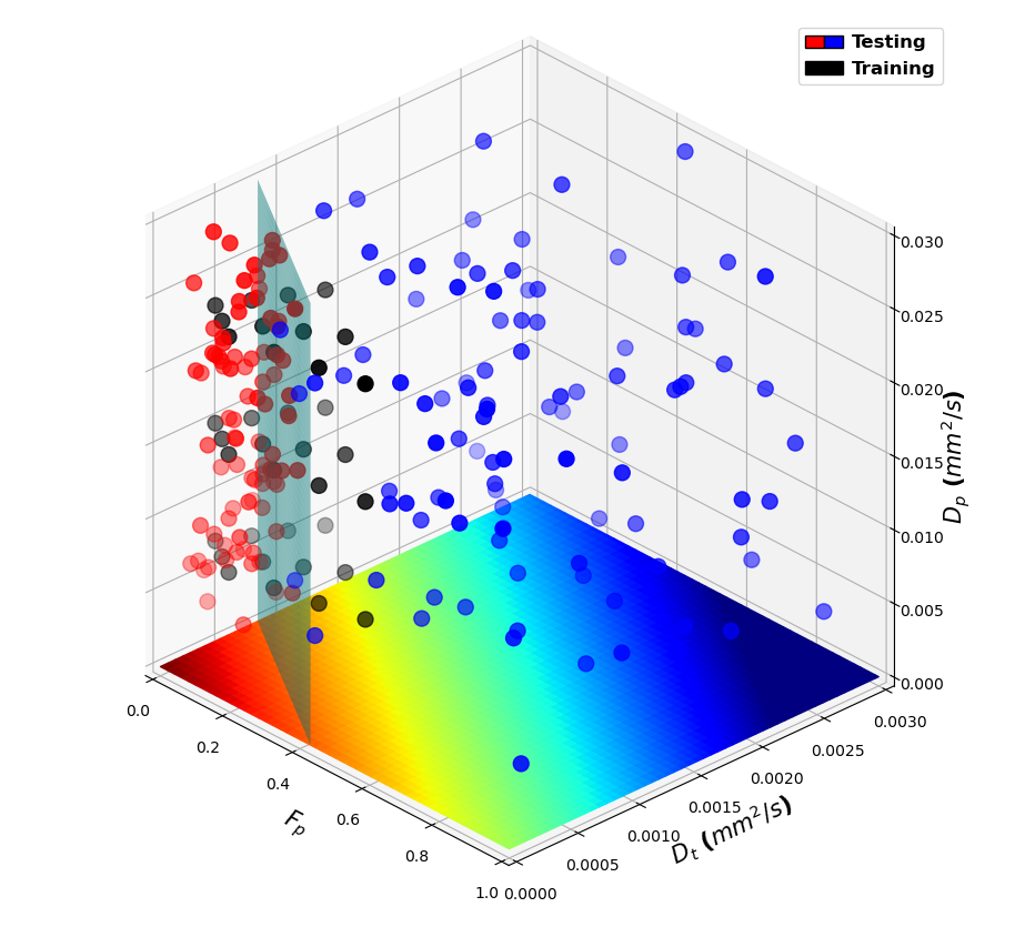
The IVIM parameters ($$$F_p, D_t, D_p$$$) are determined by a non-linear least square fitting of the DW signal decay. Considering the singular covariance matrix of these IVIM parameters, the fitting problem becomes ill-conditioned and highly affected by measurement noise^2,3. To address this issue, we formulated the distribution of estimated parameters $$$\theta_{est}$$$, given measurements $$$y_m$$$, using the following Bayesian equation(Eq. 1). Assuming that the noise follows a Gaussian distribution with a standard deviation $$$\sigma$$$, we can compute the probability $$$P(\theta_{est}|y_m)$$$ based on the DW signals measured at $$$n$$$ b-values(Eq. 2), where $$$y_{est}$$$ is the noise-free DW signals calculated with a given estimated parameters $$$\theta_{est}$$$(Eq.3). In this way, the distribution of the IVIM parameters can be calculated from the measured DW signals $$$y_m$$$ at noise level $$$\sigma$$$.$$P(\theta_{est}|y_m)=\frac{P(y_m|\theta_{est})P(\theta_{est})}{P(y_m)}\;\;\;\text{(1)}$$ $$P(\theta_{est}|y_m)\propto P(y_m|\theta_{est})=\prod_{i=1}^{n}\mathcal{N}(y_m;y_{est},\sigma)\;\;\;\text{(2)}$$ $$y_{est}=F_{p,est}*exp(-bD_{p,est})+(1-F_{p,est})*exp(-bD_{t,est})\;\;\;\text{(3)}$$
Next, we conducted LDA to separate the 3D IVIM parameter space into two tissue types, hypoxia and non-hypoxia, using histopathologically confirmed values as the reference¹(Fig. 1). We randomly selected 6 data points from hypoxic region and another 6 from non-hypoxic region, seperated by the previously defined discrimination line. Each data point was assigned with 3 different $$$D_p$$$ values ($$$8\times 10^{-3}, 16\times 10^{-3}, 24\times 10^{-3} mm^2/s$$$), and DW signals were generated based on the given $$$(F_p, D_t, D_p)$$$. Then IVIM parameter distributions were estimated based on observed signals and noise level for hypoxic and non-hypoxic data. Subsequently, we sampled the IVIM parameters from these two estimated distributions randomly(1687333 hypoxic and 3236375 non-hypoxic), forming two clusters of points. LDA was used to determine a hyperplane in the 3D IVIM parameter space to separate these two clusters. The projection of fitted IVIM parameters on the normal vector for this hyperplane is defined as a new metric, the ‘H-index’, to distinguish between hypoxic and non-hypoxic data points. For testing, we randomly picked 85 hypoxic and 100 non-hypoxic data points and classified them using the H-index. Area Under the Receiver Operating Characteristic Curve (AUROC) was calculated to assess the H-index’s performance in hypoxia classification. Furthermore, we compared H-index and other IVIM parameter maps in two prostate cancer patients with different levels of hypoxia.

Results

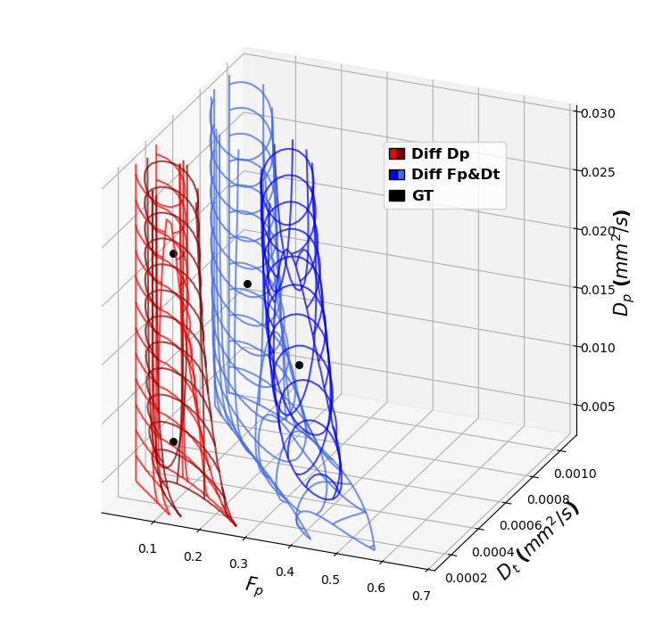
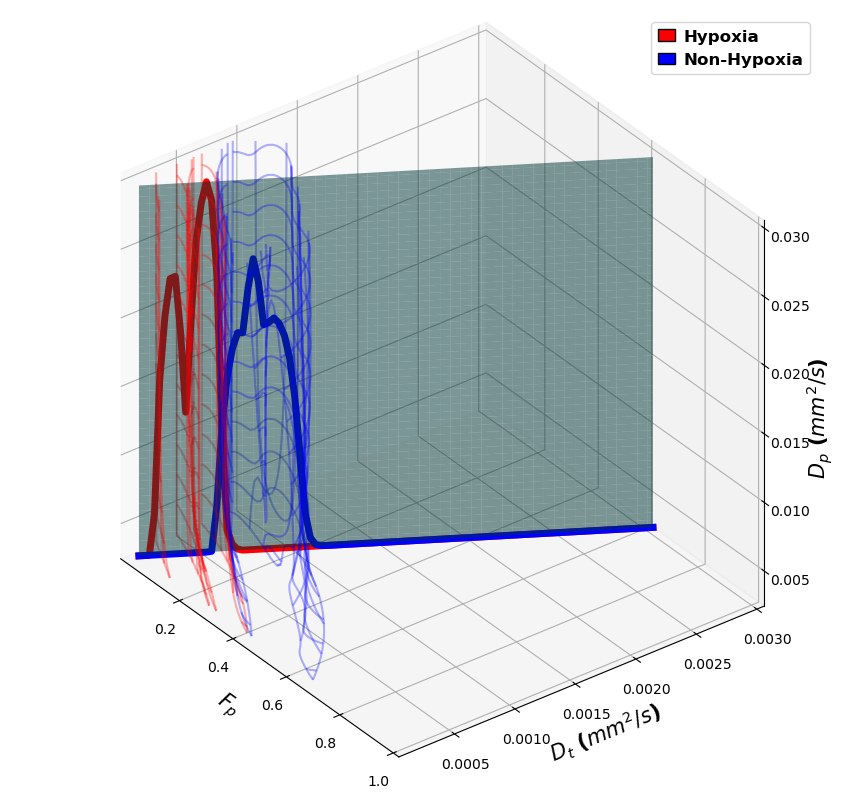
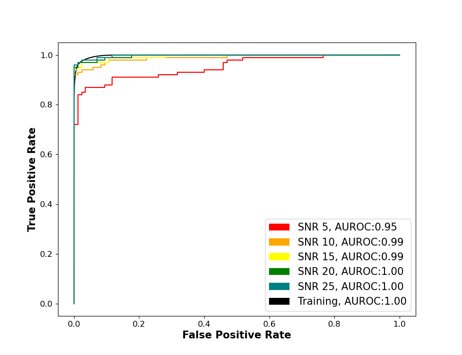
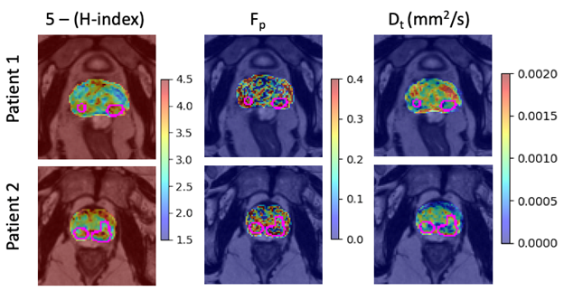
The large uncertainty in IVIM parameter estimation arises from the strong collinearity of parameters fitted by an ill-conditioned bi-exponential model. As illustrated in Fig. 2, given known values of $$$(F_p, D_t, D_p)$$$, the fitted parameter probabilities create large overlapping regions in the 3 IVIM parameters. The substantial overlap makes them challenging to distinguish from each other, resulting in significant parameter variance, especially at low SNR. The H-index, a linear combination of the fitted IVIM parameters derived through LDA(Eq. 4), effectively distinguishes hypoxic and non-hypoxic tumors(Fig. 3). This formulation aligns with the pervious study’s result $$$HS_{DWI}=K-(\frac{F_p}{0.43}+\frac{D_t}{0.79\times 10^{-3}})$$$. $$H=\frac{F_p}{0.42}+\frac{D_t}{0.79\times 10^{-3}} \;\;\; \text{(4)}$$ The H-index provided robust classification performance with AUROC = 1.00 at an SNR of 20 in the training dataset and AUROC = 0.95, 0.99, 0.99, 1.00, and 1.00 at SNR levels of 5, 10, 15, 20, and 25 in the testing dataset(Fig. 4). The classification performance remained strong at SNR levels above 5. The H-index threshold was find to be 1, matching the published work¹. IVIM maps for two representative prostate cancer patients with different levels of hypoxia and risk scores determined via biopsy are shown in Fig. 5.

Conclusion

We introduced a Bayesian-based approach to assess the collinearity in IVIM parameter fitting. Leveraging LDA, we established a robust metric for distinguishing between hypoxia and non-hypoxia prostate tumors, aligning with previous work that employed a similar equation based on diffusion MRI and histopathological correlations. Further validations of using the H-index as a tumor hypoxia indicator are warranted in future studies.

References

- Hompland, T. et al. Combined MR Imaging of Oxygen Consumption and Supply Reveals Tumor Hypoxia and Aggressiveness in Prostate Cancer Patients. Cancer Res 78, 4774-4785, doi:10.1158/0008-5472.CAN-17-3806 (2018).
- Landaw, E. & DiStefano 3rd, J. Multiexponential, multicompartmental, and noncompartmental modeling. II. Data analysis and statistical considerations. American Journal of Physiology-Regulatory, Integrative and Comparative Physiology 246, R665-R677 (1984).
- Charles, C. N. Reliability and Uncertainty in Diffusion MRI Modelling, (2016).